Machine Learning: Optimization and Community Intelligence

Summary

In a previous blog, we made note that the goal of the simple version of supply chain management (SCM) for demand forecasting in the tactical decision tier is prediction accuracy. In the wiser version, the purpose is expanded to understanding your demand which includes profiling it. Success requires the ability to mix and match a diversity of actions including a robust collaboration process that treats the forecast as a participant to continuously improve your understanding of demand and estimate the future. Two often ignored critical components of successful forecasting are the use of embedded statistical expertise to identify the appropriate statistical methods and then use optimization to determine the best parameters. Both of these functions are found in Swifcast and “Smart Forecasting”. This blog demonstrated the importance of advanced optimization for statistics (AOS) even for simple methods such as exponential smoothing and the importance of community intelligence.

Introduction

In a previous blog, we noted in the simple version of supply chain management (SCM) the goal for demand forecasting in the tactical decision tier is prediction accuracy. In the wiser version, the purpose is expanded to understanding your demand (demand profiling), bound the level of accuracy possible using demand history, and use this information to support demand and inventory analysis and put in place programs to enable the firm to adapt to changing conditions. Arkieva provides this “wiser” forecasting in Swifcast and “Smart Forecasting”. Arkieva uses a synergy of machine learning, automated intelligence, and advanced optimization for statistics (AOS) to provide this critical function. In this blog, we will provide an example of the importance of AOS to find ALPHA for simple exponential smoothing (defined below).

What is Optimization?

Optimization has two meanings for SCM: (a) getting the most out of your organization and (b) a body of mathematical methods or algorithms to find helpful information. In SCM “mathematical optimization methods” are often used in central planning and business decisions (for example COVID-19 spacing). However, they play a large role in statistics. The best known is “Best-fit straight line”. With this method, you enter or pull into Excel (or your favorite statistics software) a set of “x values” (the independent value e.g. the number of cars in a train) and a set of “y values” (dependent value e.g. the fuel cost for each train), click a few buttons and you get a “best-fit” straight line. The first part of an earlier blog on optimization has this example.

Exponential Smoothing

To illustrate the importance of AOS we will use an early and simple method of times series forecasting – exponential smoothing.

The core of exponential smoothing is predicted or estimated value is based on a weighted average of the prior actual (observed) value and the prior predicted value. The equation is:

Estimated(T+1) = ALPHA x Actual(T) + (1-ALPHA) x Estimated(T),
where ALPHA is a value between 0 and 1.
For the first time period (T=1), the estimated value is the actual value that is Estimated(1) = Actual (1).

If the current (T) predicted value is 10, the actual value is 20, and ALPHA is 0.2, the estimated value for the next period (T+1) is 12.

Estimated (T+1) = 0.2×20 + 0.8×10 = 4+8 = 12

Exponential smoothing has the following properties:

When ALPHA is 1, the estimated value is the last observation (20 in the previous example).
When ALPHA is 0, the estimated value is the prior estimate (10). In this case, the estimate for all periods is the first actual or observed value.
For other ALPHAs, the estimated value is a weighted average of all prior values where the weights decline exponentially with the increasing age of the observations.

Exponential Smoothing and AOS

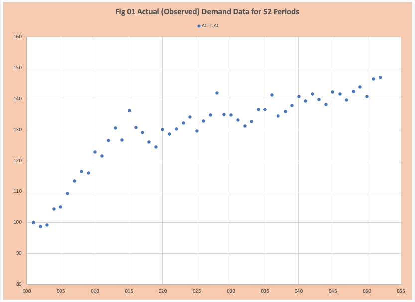
Figure 1 is a scatterplot of actual or observed demand values for 52 time periods. Some of the fundamental questions are:

What does this tell us about the demand for this product?
Is there a consistent pattern or does the pattern change over time?
What might this tell us about future demand?
What is the predicted future demand based on this time series history using a fit and predict process?

It is the 4^th question that dominates the simple view of SCM. We might start by determining how well exponential smoothing fits the data. To do that we need to decide which ALPHA to use and we will often read an ALPHA of 20% works best.

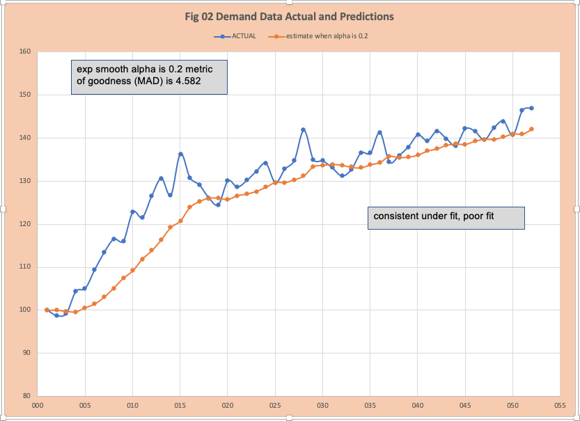
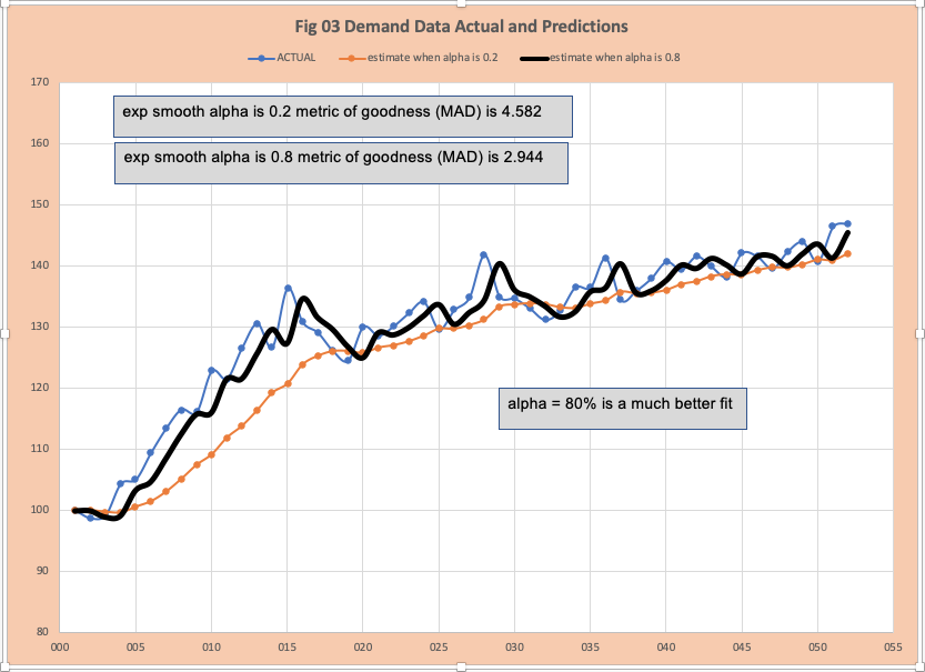
Figure 2 has the plot of the fitted values when ALPHA is 20% with the observed or actual values. The metric of goodness MAD (mean absolute deviation) is 4.582. It is clear this is a poor fit. At this point, we could easily decide exponential smoothing is not helpful and try another method. What about other values of ALPHA? We could manually try different values of ALPHA- that is a good bit of time! This is where AOS is of huge value. Applying AOS methods will identify the ALPHA = 80% (Figure 3) which provides a much better fit. There are many AOS methods that can be used to find the “optimal ALPHA”, the best known is non-linear least squares method originally proposed in 1963 in a paper by Marquardt in the journal for Industrial and Applied mathematics – well before machine learning and data science and in common use when I started doing analytics with IBM in 1977.

Insight and Demand Profiling and Community Intelligence

In the last section, we demonstrated the importance of AOS in fitting and predicting demand with respect to finding the optimal parameters (for example ALPHA) to minimize MAD. AOS also provides insight. In this example, when the best ALPHA is close to 1, this indicates most of the past history has little impact on the next period. ALPHA of 80% often indicates the last 3 periods (T-2, T-1, and T-0) have an impact on the next period (T+1). We can use this hint to drive automated intelligence to prove this insight.

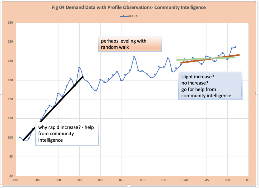
A quick visual inspection generates the following demand profile (figure 4): steep ascent, leveling, then perhaps another slight increase. This raises two questions:

How to generate this observation automatically.
The critical question of how to turn this insight into a wiser estimate of the future and adjustments to fit and predict.

For the first question, methods that use artificial intelligence in combination with statistical expertise work well. Additionally, some new AOS methods, such a joinpoint analysis can be very helpful.

The second question requires community intelligence; the people who know the product and who uses the product. We might find that early observations represent a new product introduction where there is an S-curve pattern or simply a growing market opportunity. Deciding if the last few points indicate a step increase or a temporary uptick can probably be best answered by an expert or examining the demand history of similar products.