
While reading Arkieva COO Sujit Singh’s excellent blog “Supply Chain Optimization in Supply Planning: How to Develop a New Way of Thinking”, it triggered a theme that was often helpful as software companies made the transition to optimization for supply planning from 1996 to 2001. Optimization, in comparison to rule based supply planning, has the ability see, search, and adapt to the entire and ever-changing playing field. In my previous post, I use a simple algebraic example to illustrate the key computational principle that supports important decision-making technologies.
Using Supply Chain Optimization to Make a Best-Fit Prediction
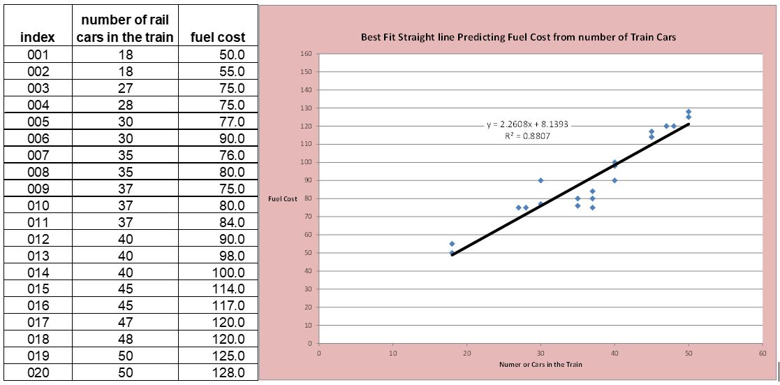
The use of optimization in supply chain management is widespread, just not in supply planning. Regular use of optimization occurs in inventory management and demand forecasting. “Best-fit straight line” is one of the most common uses of optimization. With this method, you enter or pull into Excel (or your favorite statistics software) a set of “x values” (the independent value e.g. the number of cars in a train) and a set of “y values” (dependent value e.g. the fuel cost for each train), click a few buttons and you get a “best-fit” straight line – a slope (b1), a y-intercept (b0), a measure of goodness, and a straight line drawn through your scatter plot. How is this best-fit line calculated? Does it use rules? For example, use the average of the “y values” as b0, and the slope between the smallest X value and the largest X value as b1. No, it does not use rules.
It searches.
What does it search? Conceptually it estimates a value for b0 and b1, calculates the quality of the fit by summing the differences between the predicted value and actual value, and then either stops or generates a better estimate for b0 and b1 and repeats. The algorithm for this search comes from an area of computational methods called optimization. Note “best-fit” does not mean a “good fit”; simply there are no better fits.
[Read More: Beyond the Supply Chain Maturity Model Buzz]
Let’s define search as the ability to step beyond rules and evaluate a range of solutions in a focused manner. Figure 1 shows a typical supply planning challenge involving alternative bill of material (BOM) paths to produce exit products. There are two exit products: Red Module and Blue Module where each can be produced by two different methods, and there is the potential for a shared part.
Supply Chain Optimization Techniques for Production, Inventory, and Demand
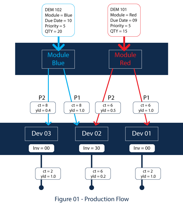
- The Red Module can be produced with process Red_P1 or Red_P2
- The P1 path consumes Dev01 with a yield of 1 and cycle time of 6.
- To get one unit of the Red Module on day 9, requires we start production of the Red Module on P1 no later than day 3 (9-6) and consuming one unit of component part DEV01.
- DEV01 requires two days to produce with a yield of 1. For this example, we will assume it does not consume any component part.
- To get one unit of DEV01 on day 3, requires we start production of DEV01 no later than day 1 (3-2).
- The Red_P2 path consumes DEV02 with a yield of 0.5 and cycle time of 6.
- To get one unit of the Red Module on day 9, requires we make two production starts (2= 1/0.5) of the Red Module on path P2, no later than day 3 consuming 2 units of DEV02.
- DEV02 requires six days to produce with a yield of 0.2.
- To get one unit of DEV02 on day 3, requires we start production of DEV02 no later than a day -3 (3-6).
- The Blue Module can be produced with process Blue_P1 or Blue_P2.
- The P1 path consumes DEV02 with a yield of 1 and cycle time of 8.
- To get one unit of the Blue Module on day10, requires we start production no later than day 2 (10-8) and consuming one unit of component part DEV02. DEV02 is shared by RED_P2 and BLUE_P1.
- The P2 path consumes Dev03 with a yield of 0.4 and cycle time of 8.
- To get one unit of the Blue Module on day 10, requires we start 2.5 (1/0.4 = 1/:=(2/5) = 5/2) units no later than day 2 and consuming 2.5 units of component part DEV03.
- DEV03 requires four days to make.
- DEV02 has inventory currently available with a quantity of 30.
- There is no other inventory.
- DEM 101 for 15 red modules due on day 9 with a priority of 5.
- DEM 102 for 20 units of blue modules on day 10 with a priority of 5.
- What set of actions should be taken to best meet the existing demand? That is matching assets (inventory and production capacity) with demand to best demand. Best is typically defined as on-time delivery, use of existing inventory, and minimizing new production starts.
- The actions include allocation of the existing inventory of DEV02 and production starts for the DEV part group?
- Is the starting point, the allocation of the existing inventory of DEV02?
Existing Inventory
Demand
Business Question
A typical rule-based approach searches one demand at a time and one alternative at a time with a priority of consuming existing inventory. It does not search alternatives.
[Read More: How do you model inventory in planning systems?]
Optimization Rule-Based Approach
- Process demand in the following order:
-
1.1. Start with the highest (most important) demand class;
-
1.2. If there is a tie in-demand class, start with the demand which has the earliest due date (within that demand class)
- When alternative BOM paths exist (for example red has a P1 and P2,
-
2.1. Evaluate (explode) the P1 path first:
-
2.1.1. If inventory exists to meet this demand, consume this inventory;
-
2.1.2. If there is no or insufficient inventory, explore the next alternative path (e.g., P2).
-
2.2. Repeat this process of looking to consume existing inventory through each alternative BOM;
-
2.3. If there is no or insufficient inventory at each alternative BOM, return to the first (P1) and generate production starts to produce the component part needed.
- Process demand DEM 101 for Red Modules first DEM 101 has the same priority as Dem102 and an earlier due date.
-
1.1. Evaluate (explode) the P1 path first:
-
1.1.1. Need 15 (since the yield is 1.0) units of Dev01 on the end of day 3 (since the due date is 9 and cycle time is 6; 3=9-6)
-
1.1.2. Inventory of Dev01 is 0, so try the next path.
-
1.2. Explore (explode) the P2 path:
-
1.2.1. Need 30 units (yield for process P2 is 0.5 need 30 to get 15 good parts) of Dev02 on day 3;
-
1.2.2. 30 units of Dev02 are available, so assign them to Dem101
-
1.3. DEM 101 will be met consuming the 30 units of DEV 02, and the supply is available on day 6 – three days early
- Process DEM 102.
-
2.1. Explode the P1 path:
-
2.1.1. Need 20 (since yield is 1) units of Dev02 on day 2 (since the due date is 10 and cycle time is 8)
-
2.1.2. Inventory of Dev02 is 0 (already allocated all to DEM101), so try the next path.
-
2.2. Exploded the P2 path:
-
2.2.1. Need 50 (since yield is 0.4) units of Dev03 on day 2;
-
2.2.2. But the inventory of Dev03 is 0
-
2.3. Return to the P1 path and explode to the next level.
-
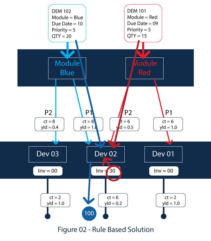
2.3.1. Need to start the production of 100 (since yield is 0.2) units of DEV02 on the day -4 (2-6). – which means will meet DEM 102 4 days later
- Results for Rule set 1
-
3.1. Dem101 is met 3 days early using path P2 and using the existing inventory of DEV 02;
-
3.2. Dem102 is met 4 days late; using path P1 and generate 100 product starts of DEV 02 (since the yield is 0.2 this produced part quantity is 20)
-
3.3. Dev 02 remaining inventory is 0; all 30 units consumed
-
3.4. 100 production starts for DEV 02 are generated
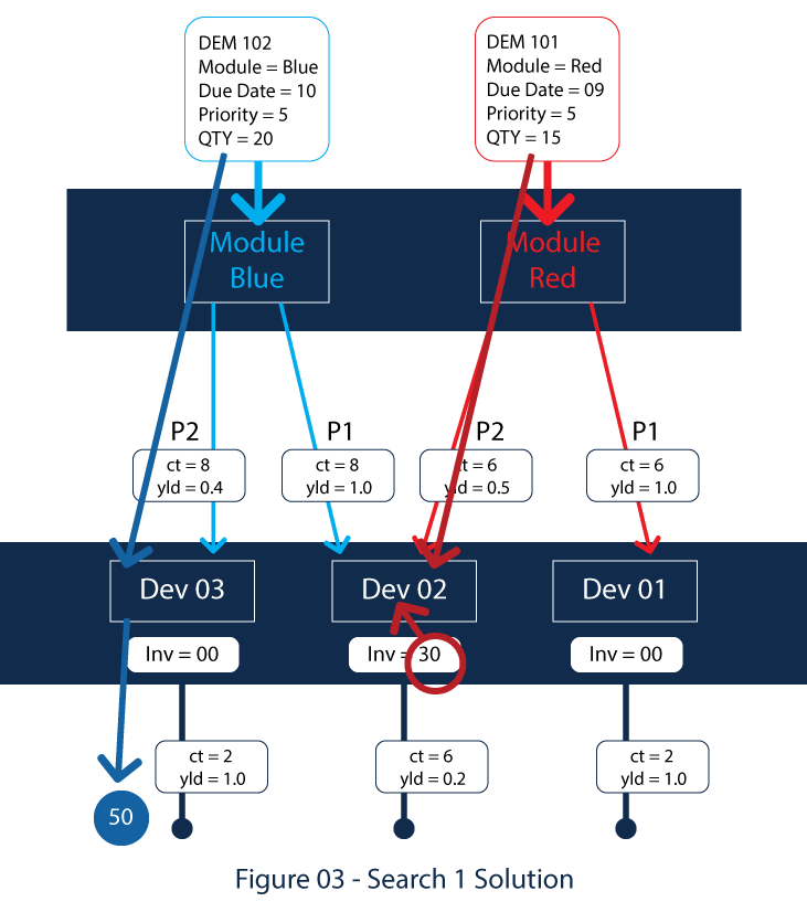
- For DEM 101 keep the same solution as in the rule-based solution.
- For Dem102,
-
2.1. Use the P2 path to produce module blue
-
2.1.1. To make 20 module blue requires consuming 50 DEV03 (50 = 20/0.4) and a cycle time of 8 days
-
2.1.2. To make 50 DEV03 requires 50 production starts (yield is 1) and a cycle time of 2 days
-
2.2. Revising the process
-
2.2.1. We start producing 50 units of DEV03 at the start of day 1, resulting in 50 good DEV03 available at the start of day 3
-
2.2.2. On day 3 we start the production of 50 units of module blue with the P2 process, and 20 are available at the start of day 11 which is one day late
- The results become
-
3.1. Dem101 is met 3 days early;
-
3.2. Dem102 is met 1 days late;
-
3.3. Remaining inventory is 0;
-
3.4. Production Starts of 50 are generated for DEV03
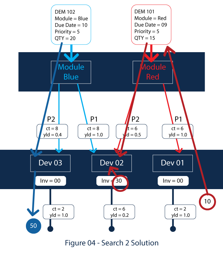
A second (and better) alternative solution is as follows:
- Allocate 20 units of the 30 units of DEV02 inventory to produce “module blue” via P1 to support DEM102
-
1.1. Since P1 has a yield of 1 none of the inventory is lost in production
-
1.2. This results in 20 units of blue module is available at the start of day 9 (1+8)
-
1.3. Which meets all of the DEM102 is met one day early
- Allocate remaining 10 units of Dev02 in inventory to make “module red” via P2 to support Dem101
-
2.1. Since the yield of 0.5, this results in 5 “module red” available at start of day 7 which is 2 days early
- To meet the remaining 10 units of demand for the red module in DEM101, do the following:
-
3.1. At the start of day 1 start the production of 10 units of DEV01 which is available at the start of day 3
-
3.2. At the start of day 3, start the production of 10 units of “module red” with the P1 process consuming the 10 units of DEV01 just produced and generating 10 units of “module red” available at the start of day 9
-
3.3. This meets the remaining portion of DEM101 on time.
- The results are
-
4.1. For Dem101,
-
4.1.1. 5 units are met 3 days early
-
4.1.2. 10 units are met on time.
-
4.2. Dem102 is met 1 days early;
-
4.3. Remaining inventory is 0;
-
4.4. 10 production starts are generated for DEV01.

[Read More: Seasonal Model Forecasting with Seasonal Methods]
This example illustrates the two sides of search
- By any reasonable metric, the solution from alternative 02 is superior to the rule base method
- The solution is “more complicated” in terms of simple rules.
The question is, can a business really afford an underperforming plan simply, so it is simple to follow?
Enjoyed this post? Subscribe or follow Arkieva on Linkedin, Twitter, and Facebook for blog updates.


