Most folks involved in Sales and Operations Planning (S&OP) for supply chain management have heard the terms “optimization” or “linear programming” with regards to supply planning and have cringed at the sound. Over the past few years a new “cringe” worthy term has emerged – “machine learning” which is sometimes used with the term predictive analytics or data mining.
The purpose of the material below is not to explain optimization or machine learning, but to provide an easy to follow example from numerical methods applied to high school algebra to illustrate the key computational principle that supports important decision technologies. We will see it as Generate,Test,Next.
To illustrate Generate, Test, Next we will use a typical problem from high school algebra involving two simultaneous equations. For the latest performance of High Octane we sold 1000 tickets and the total revenue was $7300. The cost of an adult ticket was $8.50 and senior ticket was $4.50. How many tickets of each kind were sold? (If you are thinking why didn’t you keep track of this to start – a very reasonable question) To solve this problem all we need to do is follow four simple steps:
- Investigate the problem to understand key decision and relationships. In this case this step is handled by the word problem description itself.
- Identify the decision variables – what is the unknown that we want to figure out from our detective work!
- Write a set of equations that describe the relationships between the decision variables.
- Send these equations to a “solver” that does the leg work to find the values for the variables that makes each equation “true”.
Part 2: Define the Decision Variables or Unknowns
- x be the number of adult tickets
- y be the number of senior tickets
Part 3: Write the Relationships between These Variables, Number of Tickets Sold, and Total Revenue as Two Equations. That is Translate the Word Description into a Math Description
Equation 1: handles total number of ticket relationship: x + y = 1000
Equation 2: handles total money collected: 8.5x + 4.5y = 7300
1.0x + 1.0y = 1000 (equation 1)
8.5x + 4.5y = 7300 (equation 2)
Part 4: Using a Solver to Find the Solution
To finish the puzzle, we simply need to find a value for x (number of adult tickets sold) and y (number of senior tickets sold) that makes both equations true. For this step we go visit the math genies to get a solver. As it turns out there are multiple solvers
Solver Option 1: Method from High School Algebra
In high school, you would learned a method called Symbolic Manipulation (pretty fancy term). Now in algebra you would play with these two equations to find the value of x and y that makes both equations true.
- We solve equation (1) for y
1.0x + 1.0y = 1000
y = 1000 – 1.0x
- Substitute the equation for y into equation 2 and solve for x
8.5x + 4.5y = 7300
8.5x + 4.5(1000 – 1.0x) = 7300
8.5x + 4.5(1000) – 4.5(1.0x) = 7300
8.5x + 4500 – 4.5x = 7300
8.5x – 4.5x = 7300 – 4500
4.0x = 2800
x = 2800/4 = 700. - Use the value for x (700) to calculate y
y = 1000 – 1.0x
y = 1000 – 1.0(700) = 1000 – 700 = 300
The answer is 700 adult tickets (x) and 300 senior tickets (y) were sold, when we put these values into equations (1) and (2), we find both are true.
The two equations are:
1.0(700) + 1.0(300) = 1000 (equation 1)
8.5(700) + 4.5(300) = 7300 (equation 2)
Solver Option 2: Gauss-Seidel method (Better for Computer)
- We take the 2 equations previously defined and solve one for x and the other for y
The two equations are:
1.0x + 1.0y = 1000 solving for y: y = 1000 – 1.0x (eq 1)
8.5x + 4.5y = 7300 solving for x: x = (7300 – 4.5y)/8.5 (eq 2)
With these two equations we “Generate, Test, and Next” – let’s look at the details.
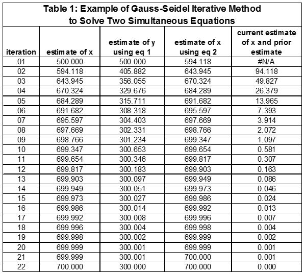
- We generate an initial estimate of x (number of regular tickets sold). Often any estimate works, we will use some reasonable value, in this case 500 since the total number of tickets sold is 1000.
- We use this value for x (500) and equation 1 solved for y (= 1000 – 1.0x) to calculate 1. We have y = 500 (=1000 – 500).
- We use equation 2 to generate a new estimate for x from equation 2 solved for x. This value is 594.117 (= (7300 – 4.5(500))/8.5).
- We compare the old estimate for x of 500 with the new estimate of x (594.118) calculate the difference which is 94.118 (= absolute value of (500 – 594.118).
- We test, if the difference is small enough, we stop. If the difference is large, we go to next – generate another estimate of x, repeating the process above.
- We solve for y using the new estimate of x. y= 405.882 (=1000 – 594.118), then solve for x using equation 2, generating a new estimate for x which is 643.995.
- This continues until the difference between the successive estimates of x is small enough.
- Or this method does not “converge” – a fancy terms for not working. A topic for another time!
Table 1 has the result from 22 iterations.
Like this blog? Follow us on LinkedIn or Twitter and we will send you notifications on all future blogs.