What-if Wednesday: Seasonal Model Forecasting with Seasonal Methods

In the previous blogs, we experimented with different variants of Holt Winters method. This time we will be analyzing forecast simulations using Seasonal and Robust Seasonal methods with the same data set.

Seasonal method is a regression method that fits a linear trend along with sine and cosine curves. These sine and cosine portions of the regression can fit any seasonal deviations from the linear trend. Robust seasonal method also fits a trend along with sine and cosine curves, however, this method uses linear programming to fit a seasonal series in a way that compared to the regular seasonal method is less likely to be thrown off by noisy values that depart from the trend or seasonality. Robust seasonal method tries to minimize mean absolute deviation (MAD) rather than squared error since MAD is less influenced by individual outliers.

[Read more: Statistical Forecasting with Damping Factors]

Seasonal Model Forecasting Results

Unlike the Holt Winters method, these two methods do not have alpha, beta and gamma parameters. Seasonal method has two parameters: Regression Weight and Damping factor. Robust seasonal method, in addition to the seasonal method parameters, has penalty parameters. These penalty parameters refer to additional effects that the method is capable of estimating. These can detect a level shift where there is a one-time increase or decrease in the overall level of the series. They can also detect if there is a single month where the series has a seasonal adjustment that departs from the sine and cosine curves that the model is trying to fit.

Shown below are some of the simulations we ran using the history data as shown in the first chart.

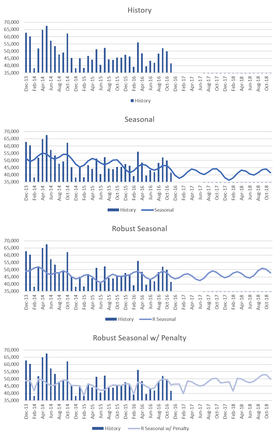
Seasonal method: The second chart above shows the forecast using the seasonal method with a default regression weight of 0.97 and damping factor of 0.85. We see that the forecast has the cyclic variations in the form of sine and cosine waves which capture seasonality along with the decreasing trend.
Robust seasonal method: The third chart above has the forecast using the robust seasonal method with default parameters. We see that the forecast it generates follows the general sine and cosine form but unlike seasonal method robust seasonal forecast is less aberrant from the trend. Also, the forecast here is noticeably higher than the seasonal method. This is because early history has larger values and seasonal method is trying to fit a downward trend. Robust seasonal probably put a downward level shift after the early history and then fit the recent history with a somewhat upward trend. Also, low Feb values were possibly pulling down the surrounding values when it could only be fit with a sinusoid.
Robust seasonal with penalty: The last chart shows the robust seasonal forecast where we have altered a parameter to allow penalty for a single month that departs from the regular sine and cosine curves. Since the month of February has lower than normal historical values the method chose that month to apply the penalty. Accordingly, the forecast for February month is also lower for the next two years.

[Read More: Forecasting Methods]

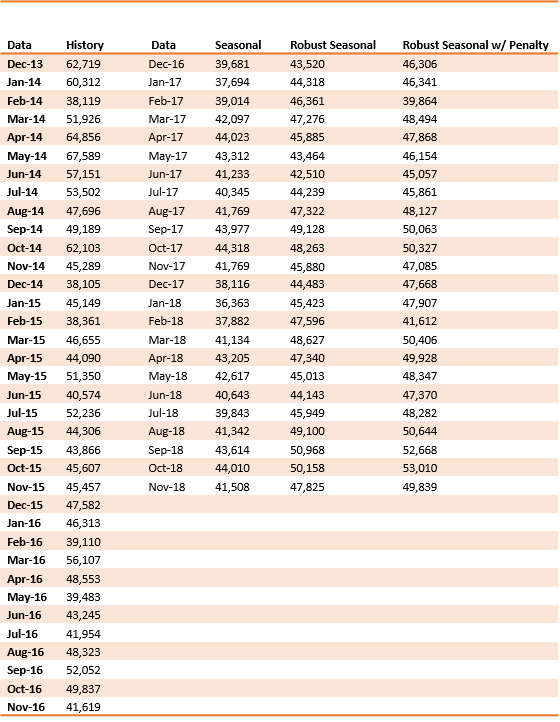
Either the seasonal or robust seasonal can be used with sufficient history. Although we fit with a 12-month cycle, two or more years’ data is advisable. These methods would be most effective with long-term stable trend. For example, in case of consumer-packaged goods. The exact numerical values of the forecasts generated above are available in the table below.