Introduction
In a recent discussion, I observed that the operating curve made it clear the wrong inventory approach could strangle production output.
The successful measurement and management of inventory remains a hot topic in supply chain management in 2022. Like a fever, it is easy to measure but the cause may be complicated since it is “collateral damage” of all supply chain management (SCM) decisions – even those far away such as what data to use for historical demand. The easiest path is to use the standard formulas for safety stock, set arbitrary targets, and edict reductions in inventory. In fact, inventory has multiple realities where success requires that ability to model the demand supply network (DSN).
Although inventory is challenging to manage, it can and is an indicator of a runaway train. Sales folks lobby to have their favorite demand put into the forecast just in case; at the slightest hint of a shortage the raw material planner will double their order. Factories are troubled by unused capacity and will easily take the path: “on a hunch, start a bunch”.
What is the Operating Curve (OPCURVE)?
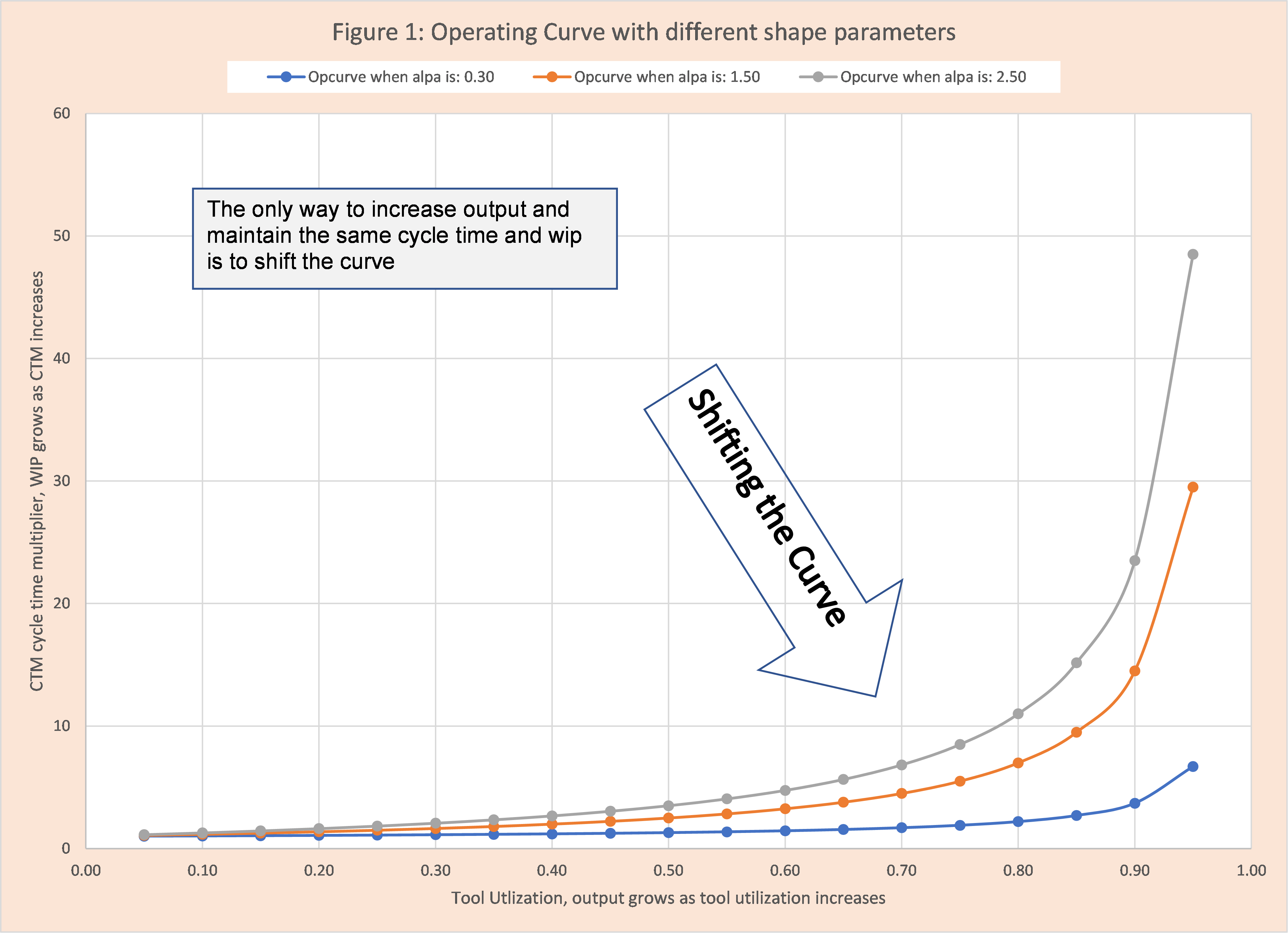
When variability exists, either in arrivals or services, there is a trade-off between server (machines, people) utilization and the cycle time to complete an activity or service. The higher the utilization, the longer the cycle time for a fixed amount of variability. The curve (relationship) that describes this trade-off is called the Operating Curve (OPCURVE) and typically as tool utilization increases the cycle time increases. Often, the relationship is a monotonically increasing non-linear function (figure 1). This relationship between cycle time and utilization applies to factories, banks, grocery stores, help desks, emergency rooms, etc. – there is no hiding from it. This relationship and the curve follow naturally from queuing theory equations as well as empirical observations.
How does this relate to inventory?
Cycle time is divided into two components: wait time and raw process time (RPT). Wait time requires the accumulation of a special type of inventory called WIP (work in process) within the production or service flow. Think about paying for your groceries at the local market. There are two components: waiting for the cashier to process your order and the actual checkout process. The time it takes to check out is the RPT. Often the RPT itself can be broken down into components. Again, let’s look at paying for groceries. There are four major activities: putting your groceries on the belt, the scanning process of each item to determine your cost (and for inventory), bagging the groceries, and paying for the groceries.
The challenge for inventory
Net is to get more output from production, requires higher tool utilization, which requires additional wait time, which requires additional WIP (special type of inventory). This drives two management challenges:
- What is a reasonable amount of WIP to expect given the current operating situation of the factory?
- What steps can be taken to reduce variability and shift the curve?
In the next section we will provide a simple example of WIP expectation (challenge 1). Challenge 2 is outside the scope of this discussion.
WIP and Production
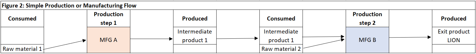
We will use the following very simple production sequence to illustrate the relationship between WIP and production output.
The core production flow is illustrated in figure 2. This is discrete manufacturing. The first production step (MFG A) consumes raw material 1 and produces intermediate product 1 which is then placed into storage – its only purpose is to be component product to be in used in the second production step (MFG B). MFG B also consumes raw material 1 and produces exit product LION.
Production Step 1 (MFG A) has the following characteristics:
- There is just one tool or resource dedicated to this production.
- It processes one widget at a time, there is no lot size.
- This produced widget (intermediary product 1) is put into storage to be consumed in MFG B
- Its raw throughput per hour, or production rate, is 10. If the tool is available, MFG can produce 10 widgets per hour.
- The time to produce one widget is raw process time (RPT) and this is 0.1 hour (=1/10) or 6 minutes.
- Its availability fraction, or percentage, is 60%. This has two related interpretations:
- When I decided to produce a widget at MFG A, the chances the tool that does this work is working properly is 60% and the chances the tool isn’t working is 40% (=100%-60%).
- On average, the tool is available only 60% of an hour or 36 minutes.
- The effective throughput is 6 (=10 x 0.6).
- Effective throughput is defined as raw throughput per hour (10) times the availability (60%).
- The justification is for any given hour the tool is only available for 60% of the hour (36 minutes). The throughput for these 36 minutes is 10 per hour. For the other 40% of the hour (24 minutes) the throughput is 0. Therefore, the actual production is (10 x 0.6) + (0 x 0.4) = 10 x 0.6 =6.
- The effective raw process time (RPT) is 0.1667 hours (=1/6) or 10 minutes.
Production Step 2 (MFG B) has the following characteristics:
- There is just one tool or resource dedicated to this production.
- It processes one widget at a time, there is no lot size.
- This produced widget (exit product LION product 1) is put into storage to meet demand.
- It’s raw throughput per hour or production rate is 6.
- The time to produce one widget is raw process time (RPT) and this is 0.1667 hour (=1/6) or 10 minutes.
- Its availability fraction, or percentage, is 90%.
- The effective throughput is 5.4 (=6 x 0.9).
- The effective raw process time (RPT) is 0.1852 hours (=1/5.4) or 11.11 minutes.
The key decision controlling the WIP inventory level is when to start one unit of production at MFG A. Which decision is best?
- The bright, young data science professional with a brown belt in Lean recently hired by the CFO to ensure manufacturing follows the science and not tribal folk lore immediately observes inventory is minimized with the following start decision:
- A unit of production at MFG A is started only when a unit of production at MFG B is started. In fact, one could offset the start at MFG A by one minute. The proof is obvious – MFG A can produce one unit of intermediary product in 10 minutes, which is faster the effective RPT of 11.11 for MFG B. Therefore, just-in-time management insures almost zero WIP inventory.
- The brand-new finance MBA immediately concurred with the data scientist and did a quick calculation in Excel to estimate the financial improvement associated with this rule.
- A seasoned manufacturing production leader speaks up and says historically production attempts to keep 1 or 2 units of intermediary product 1 in inventory to protect against production variation.
- The rule is when the inventory level intermediary product 1 drops to 1 or 2, a unit of production at MFG A is started.
The seasoned production leader is immediately challenged with a good bit of hostility. Some of the comments were:
- There is no data science in your decision
- It is obsolete tribal knowledge
- This is why inventory is out of control
As the meeting was about to end and the CFO had concurred with the recommendation, an aged stranger moved with slow and noiseless steps up the main aisle carrying two books, his body clothed in a brown robe that reached to his feet, his face unnaturally pale. He then asked these questions:
- How often will MFG B be ready to produce an exit product (LION) and not have an intermediate product to consume? That is, how often will “idle” without part occur?
- What is the loss of output associated with inventory savings?
- What is the impact on customer satisfaction and market growth?
The stranger then left two books on the table, Hillier and Lieberman Operations Research and Factory Physics, and left almost instantaneously out a back door. Additionally, there was one printout of a Monte Carlo simulation program using weird symbols and the estimate of lost production of 12 units per day. The audience was now certain the man was a lunatic, and the books were immediately burned.
A few months later, after the new inventory control policy was put in place and output fell, driving reduced revenues and loss of market share, the three standard criminals were arrested and verbally flogged. New AI efforts were started to improve performance.
Conclusion
Managing inventory and finances is critical for the success of every firm and it is a challenging job to reduce unnecessary spending and drive an efficient organization. Data science is a very effective decision technology for some situations. However, in every demand supply network (DSN), complexity exists whether you ignore it or not – best not to ignore it. Success requires facilitating community intelligence and core methods from Operations Research.