The main objective of demand forecasting is to help a business better prepare to meet demand. An over forecast could lead to an overstock and increase in inventory costs while under forecasting could lead to stock outs and missed business opportunities. As such, having a more accurate demand forecast by selecting the right demand forecasting method can directly translate to saved costs or an increase in revenue.
Here’s what we’ve discovered after comparing the accuracy of different demand forecasting methods.
In the last few months, we ran simulations using various seasonal methods. We started experimenting with Winter’s additive method by adjusting its alpha, beta and gamma parameters. Then we analyzed the forecast generated from Winter’s multiplicative method by varying its alpha, beta and gamma parameters. Finally, we used seasonal and robust seasonal method to study the forecast. The historical data that we used for this entire exercise was the same across all the different methods used.
Analyzing the Forecast Accuracy for Different Forecasting Methods
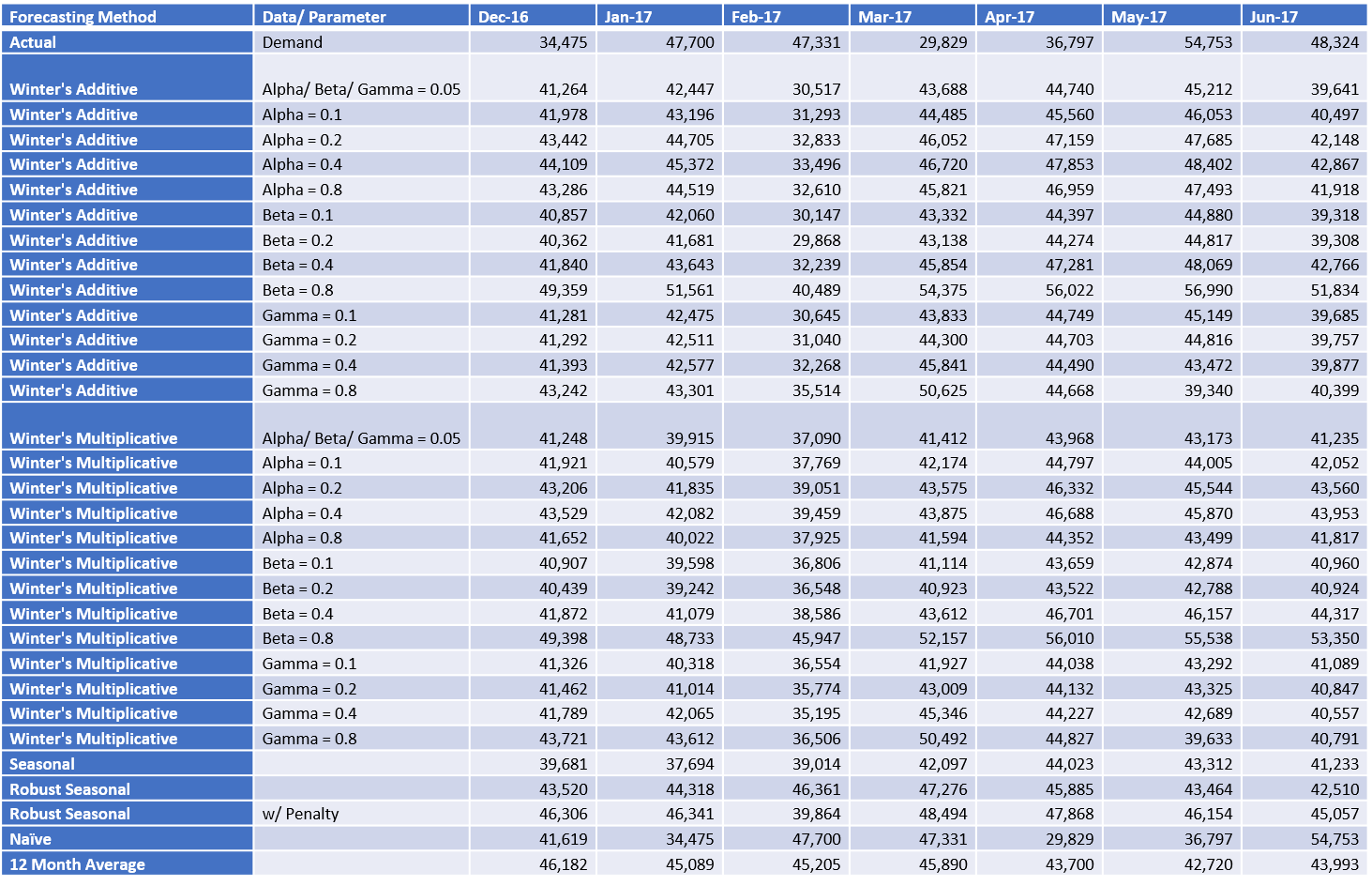
In this blog, we are going to analyze how accurate the various forecasting methods were in predicting future demand. The historical data set that we used for generating the forecast ranged from Dec 2013 to Nov 2016. So, we took the actual demand from Dec 2016 to Jun 2017 and compared it against all the different forecasts generated previously. We also added Naïve forecast and last 12 Months Average forecast in the comparison table to see how good the other forecasting methods are relative to these basic methods.
Below is the table that shows the actual values of the demand for the 7 months and what we forecasted using various methods in the last few months of our simulation.
We calculated the accuracy of all these methods by using the mean absolute percent error (MAPE) formula.
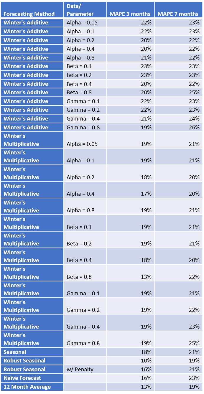
Two sets of MAPE were calculated; one for 3 months (Dec, Jan and Feb) and another for 7 months (Dec through Jun); to gauge how accurate these methods were in predicting next 3 months (short term) and next 7 months (long term).
[Read More: The Family Tree of MAPE]Below is the table with respective MAPE values in percentage:
We see that almost all the methods have an error rate less than 25%. Predicting next 3 months was more accurate (19% MAPE on average) than the next 6-7 months (22% MAPE on average). Using very high values of Beta (trend parameter) and Gamma (seasonality parameter) parameters in Winter’s method have a negative effect on forecast (MAPE was higher as compared to lower values of these parameters). However, the difference was not significant to necessarily say that increasing the parameters would always be negative. One can pick a reasonable value and let it be.
Seasonal, Robust Seasonal, Naïve and 12 Months Average methods in this dataset yielded comparatively lower MAPE. One could say that using the Winter’s method made the forecast worse as compared to using a simple Naïve or 12 Month Average method. Robust Seasonal method was the one that gave the least error in predicting the next 3 months as well as the next 7 months.
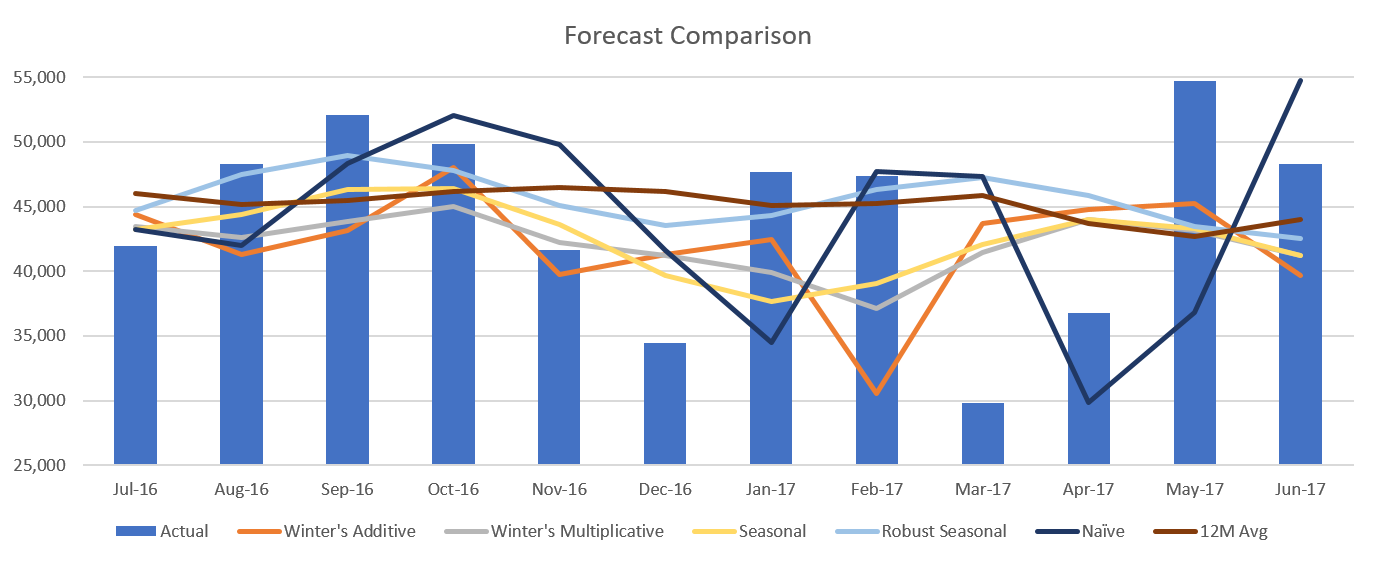
[Read More: Three Steps to a Better Statistical Forecast Setup]The chart below shows the actual demand along with what Winter’s Additive, Multiplicative, Seasonal, Robust Seasonal, Naïve and 12 Months Average forecasts.
We know that the forecasts are almost never accurate but overall if for the next 3 or 6 or even 12 months if choosing a right forecast method could give a 10 percent reduction in the error (choosing Robust Seasonal vs Winter’s additive for this data set for example) it could mean a lot of savings for the business. Also, one should keep in mind that the methods that look good to the human eye (Winters for example) may not always be the best when it comes to the metrics.
[Read More: 5 Steps to a Better Statistical Forecast ]Enjoyed this post? Subscribe or follow Arkieva on Linkedin, Twitter, and Facebook for blog updates.


