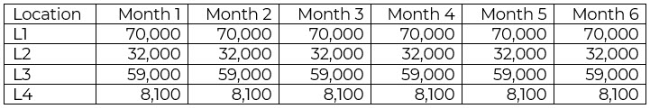
I was reviewing a supply planning spreadsheet from a contact recently. This contact had multiple factories, and each factory had multiple manufacturing resources or production units. However, the capacity field of the spreadsheet was populated with a constant value representing max number of units that could be produced in each period (imagine max capacity being a straight line on a graph). This looked like the table below.
Now this made me curious to say the least. Why would the capacity number not go up and down with months? For starters, different months have different number of days in them. Further, the factories themselves were of different vintage, with the older ones prone to more frequent breakdowns, and different machines had different capabilities. I did check and confirm with them that the rate of output could go up or down depending on the product that was being made on a particular machine. In other words, the mix of products mattered in determining how much output the factory would be able to generate. And this was a seasonal business. The mix of demand changed with the seasons and in fact with every period in question. At a product family level, the demand at one of the locations looked like the graph below. As you can see, the mix in demand changes monthly.

On a percentage basis, the same data looked like the graph below. As one can see, the demand for all families moves around, and product family 1 shows a clear month over month decline in demand.

Let us say that in the example above, Product Family 1, which has the least demand, takes the longest to make. Say it runs at 1/10th the average rate of the other product families. This would mean that in Month 1, the total output would be considerably less than month 6 as the demand for product family 1 is a lot higher in month 1 compared to month 6. Producing equal to the demand in month 1 would use up a lot of capacity and leave little room for the other product families. Ken has described this math in some detail in this blog.
The question then is: With the mix in the demand varying quite a bit from month to month, and with the run rate on the manufacturing resources being different for different products, is it acceptable to use a flat line as the max capacity? Or should we use something more nuanced? And what should that nuanced version be?
The answer depends on what software tools and data are available. If the tool at hand can calculate capacity used on a time basis, then that would create the ideal scenario where one would model capacity in units of time. As an example, for one manufacturing resource, assuming a 24 X 7 operation:
- Maximum Available Capacity = Number of Hours in a Period
- (= 24 * 30 in a 30-day period)
- Capacity Used for One Product = Run Rate (in Hours / Unit) * Number of Units Produced (of said product)
- Total Capacity Used = Sum of Capacity Used by All Products Being Made (on the resource in question)
- Capacity Unused = Maximum Available Capacity – Total Capacity Used (on the resource in question)
This type of mix-based modeling of capacity allows a more precise calculation of the capacity used. It further allows modeling capacity lost in changeovers, restarts, maintenance, etc. Of course, the requirement to do this type of modeling is to have access to tools that can handle the slightly more laborious (but not difficult) math. Folks in process manufacturing would probably never plan capacity without considering mix. Folks in discrete industry might be able to get away with a unit level representation of capacity.
Let me close this discussion by going back to the original spreadsheet the contact mentioned above. The contact was from the process industry and acutely aware of mix issues, as well as time lost in changeovers. Further, they also said that two of the factories were so old that too many changeovers caused resources to breakdown which further reduced the capacity.
Why then were they using a simplified representation of capacity in units? The answer was simple and pragmatic. While they agreed that the calculation would be more precise if done the way I have described above, they did not feel that it would necessarily help the business any. In their words, the forecast accuracy was less than 50%. So, with the main driver of the model being that far off, what difference would it make if they updated the Excel model to calculate the capacity used more precisely? Their plan was to work on and improve the forecast accuracy before investing in a more sophisticated supply planning model. They were OK with using an average number for now. They were very clear on not confusing precision in the underlying calculation for more accurate or better results.
It is difficult to argue with clear headed logic like that. Plus, it aligns with the steps of the implementation methodology advocated by Arkieva:
- Understand customer demand
- Understand inventory
- Create a demand plan
- Create a supply demand balancing model
- Create and run a sales and operations planning process
If you are dabbling with supply and capacity planning, consider these thoughts as you make the decision on how to do it. If you need a supply planning tool that can crunch the numbers at a more detailed level that does include the mix, reach out to us at Arkieva.