One value of supply chain modeling is the ability to explicitly model capacity or constrained resources. Which products get what capacity in what amount at what time? How does this impact on-time delivery? Where do I add capacity? These types of questions are custom made for a “little bit of math” and difficult to do in a simple spreadsheet model. Simply put think about attempting to pick a “best fit” straight line for a set of data without using “a little bit of math”. Folks would argue all day about which “line” fits best. In this blog we will look at one example from semiconductor manufacturing and one from chemicals.
The core of handling resource allocation in supply chain modeling is linking a manufacturing activity to one or more resources. Normally this is done by associating a consumption rate for each unit of production by that manufacturing activity for the selected resource and the total available capacity for the resource.
Wafer Fabrication, Capacity, and Supply Chain Models
Let’s consider the production of widgets. Each widget needs to be processed through six operations in sequence 101, 151, 201, 202, 301, and 302. Table 1 tells us which tool can service which operation at what rate. Operation 101 and 151 can be handled by Tool A and B. Operations 201, 202, 301, and 302 can be handled only by Tool A. Observe Tool A can service all 6 operations, but Tool B can only service operations 101 and 151. Tool A and Tool B are each available for 1152 units per day.
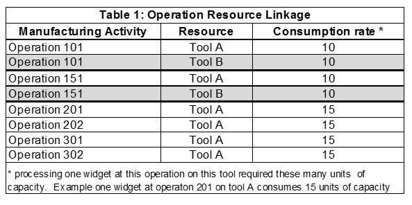
Assume for simplicity, we have a uniform start rate of 10 widgets per day, where Tool B exclusively services operations 101 and 151 and Tool A exclusively services options 201, 202, 301, and 302. In steady state each operation would process 10 widgets per day.
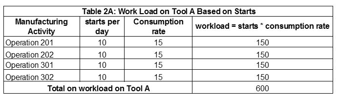
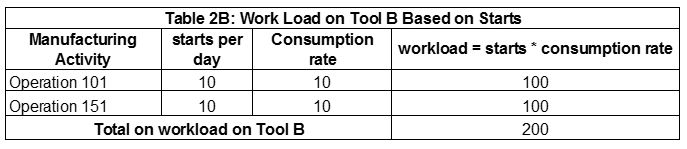
What capacity or workload is needed for each tool to meet the daily required production from this start pattern? The daily workload on Tool A is the sum of the workload on the four operations it services. This calculation is illustrated in Table 2A (600 = 10 x 4 x 15. The daily workload on Tool B is provided in Table 2B (200 = 10 x 2 x 10). Since Tool A and Tool B have 1152 units available each day, there is plenty of capacity to support this demand.
Quickly the question that arises is given this available capacity what start rate can the factory support. The answer is between 19 (=1152/ (4×15), where the capacity of Tool B is the limiting factor (1140 = 19 * 4 *5). If demand for widgets rose to 30, our supply chain model would indicate this was not feasible (short fall of 600 units of capacity for Tool B) and we should either reject the increase or attempt to delay the delivery date.
However, what the model lacks is access to the tactical deployment decisions or decision hierarchy. In wafer fabricators often a tool can, in theory, handle many different operations but at a given point in time is only actively deployed to a small subset of these operations.
This “reduced” deployment occurs for a number of reasons, including:
- It is physically impossible for the tool to be “actively” ready for more than a small number of operations. If we want the tool to handle an operation differently than the currently selected number, the tool has to be brought down for a while, “retooled”, and brought back up
- There are manufacturing performance advantages to limit the number of operations a tool is currently deployed to handle
- The manufacturing team often uses deployment decisions in an attempt to “balance” tool load by “guessing ahead”
- The manufacturing team prefers to deploy its fastest tools to certain operations to keep total cycle time low
- Habit or prior practice
What occurs is the tactical deployment decision made by manufacturing when reflected in the capacity information used by the supply chain model which in fact understates the real flexibility of manufacturing to produce widgets to meet an increase in demand. Often, the allocation of Tools to operations is based on a recent manufacturing mix of products, and not necessarily on what the market is demanding.
In our example, it might well be that there is an older tool, Tool C, which can, after being retooled, be switched from working on “gadgets” to widgets — specifically it can handle operations 201 and 301. This is reflected in Table 3.
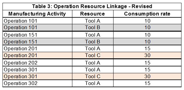
Tool C is not as efficient as either Tool A or Tool B, but for this particular mix of widgets, it can dramatically increase the total capacity needed for the current demand. Manufacturing is reluctant to use Tool C in its mix because the tool is less efficient (its consumption rate is higher per operation) than Tool A. Ultimately the purpose of manufacturing is to optimize the delivery of product, not internal measures of efficiency.
We might be tempted to state the old adage – garbage in garbage out – in fact that would be wrong and fail to understand the environment that generated the “limited” but accurate capacity information. In fact, the capacity information provided by manufacturing to the supply chain model as reflected in Tables 1 and 2 was accurate, but limited. It was limited to the current near term production requirements and the near term ability to use the tools. Tool C cannot be used for operations 201 and 301 until it is “retooled” and qualified. This may take a day or it may take a week – but certainly manufacturing cannot afford to “retool” on a daily basis.
Continuous processes and varying rates
Another example where a “little bit of math” may be useful is in continuous chemical processes. Consider a reactor that used a catalyst bed for reaction. Catalyst beds tend to “gunk” up over time and need to be renewed. Fortunately, they degrade over time. As the catalyst bed degrades, the production rate falls off. In some instances, the yield falls off too. What this means is that as the catalyst gets older, not only can you make less per day, but the percentage of good stuff versus bad stuff decreases as well.
Let’s consider an example where the production rate per day when the catalyst is fresh is 10 tons per day, it takes 0.5 days to renew, and production rate that the catalyst can support decreases by 0.15 tons/ per one half a day, each half day the catalyst is used.
In the simplest case, we renew the catalyst each day, which means the reactor, only runs for half a day. It starts the period with a rate of 10 tons per day and ends at the rate of 9.85 (=10 -0.15) tons per day for an average rate of 9.925. Since the reaction only ran for one half a day, the effective production rate per day is 4.96 (=9.925/2) tons, creating an effective rate of 5 (=10×0.5) tons per day.
What if we renew every two days? The rate at the start of period is 10 and the rate at the end is 9.55 (there are three one half days in this period, so the total loss is 3 x 0.15 = 0.45, 9.45 = 10.00 – 0.45). The average production rate is 9.78 = ((10.00 + 9.55)/2). The total production over two days is 1.5 x 9.78 = 14.66; which makes the average production per day 7.33 tons per day. Table 4 and Graph 1 show the relationship between average daily production or effective capacity and the days between renewal of the catalyst.
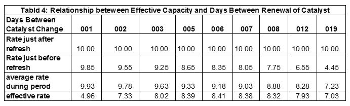
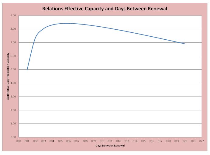
The “optimum” policy is to change the catalyst every 6 days. But in reality, the decision as to when the catalyst should be changed depends on the availability of the maintenance crew, the need for critical production, the type of product being run and a host of other factors. In this particular case, it may not matter much because the catalyst seems to degrade rather slowly anyway. It is straight forward to include the loss in yield and will leave that an exercise to the reader.
When manufacturing provides a rate to be used in planning, it usually reflects an achievable rate, and not necessailly a realistic rate given the current mix of products. To overcome this, some planning advocates suggest using a “demonstrated” production rate. This is certainly different from the maximum achievable rate, but in reality is no more accurate.
For more information please see:
Fordyce, K., and Milne, R.J., (2012), “The Ongoing Challenge for a Responsive Demand Supply Network: the Final Frontier—Controlling the Factory,” chapter 3 in Decision Policies for Production Networks, edited by Armbruster, H.D. and Kempf, K. Springer. pp. 31-70.
Fordyce, K., Milne, R.J., and Singh, H. 2012, “The Illusion & Complexity of FAB Capacity in Central Planning the Ongoing Challenge – Tool Deployment and the Operating Curve”, invited paper and presentation, MASM 2012, Winter Simulation Conference.