Introduction
This is one of the top 5 questions in supply chain management (SCM) from demand planners to the VP of supply chain. The folks in the trenches want a definitive answer – give me a simple metric that I can use in all cases that provides guidance. They do not want the academic cop out – “it depends”. Pulling from my experience in the trenches (three IBM Outstanding Achievement Awards) and an academic background (over 30 publications in refereed journals), I will outline a few key tools of the trade to assess “forecastability”. These “key tools” balance a need for simple with a need to handle the complexity of SCM – following the IBM adage – complexity exists whether you ignore it or not, best not to ignore it. This topic is covered in more detail in a recent Arkieva webinar. The methods and tools described here are part of Arkieva smart forecasting and will reveal two key lessons:
- A critical component of forecastability is the tools you have in your tool kit.
- The forecastability is limited by the inherent variability in the process generating demand.
Which Data
Demand management encompasses many functions and involves a rich set of data that is often aggregated and disaggregated and involves mixing judgement with statistics. For this discussion, we are focused on the analysis of a single historical set of demand data – called a time series. The time series may be at any level of aggregation. For example, if the historic demand data is actual sales of soap where we have soap SKU, date, quantity, soap type (each soap SKU belongs to one soap type), type of sale (store or online), location of the store, and geographic region where the store is, you might want to estimate demand at the soap SKU level by store and internet. Perhaps at the soap type level. These decisions are part of establishing your forecast pyramid or strategy.
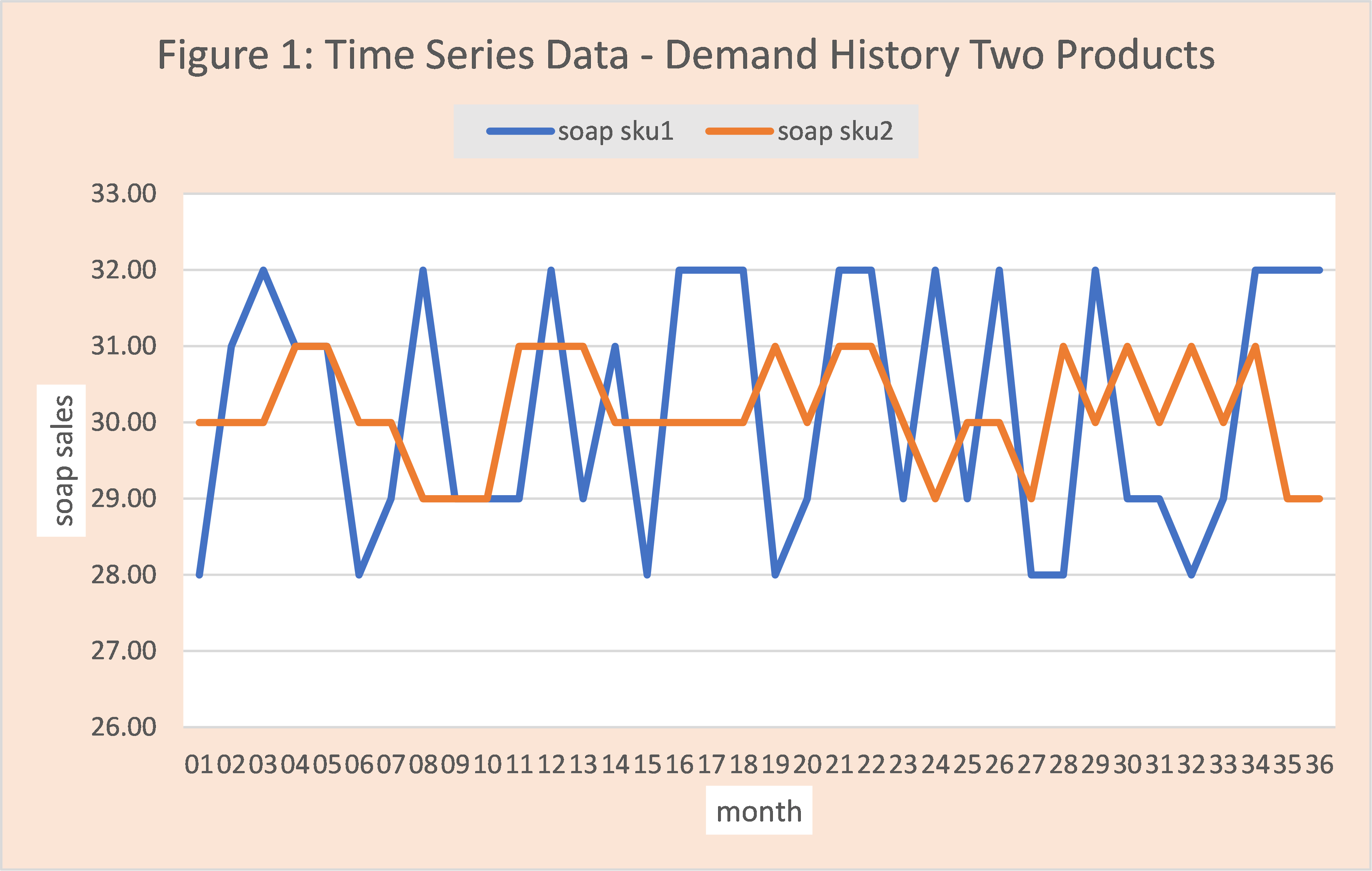
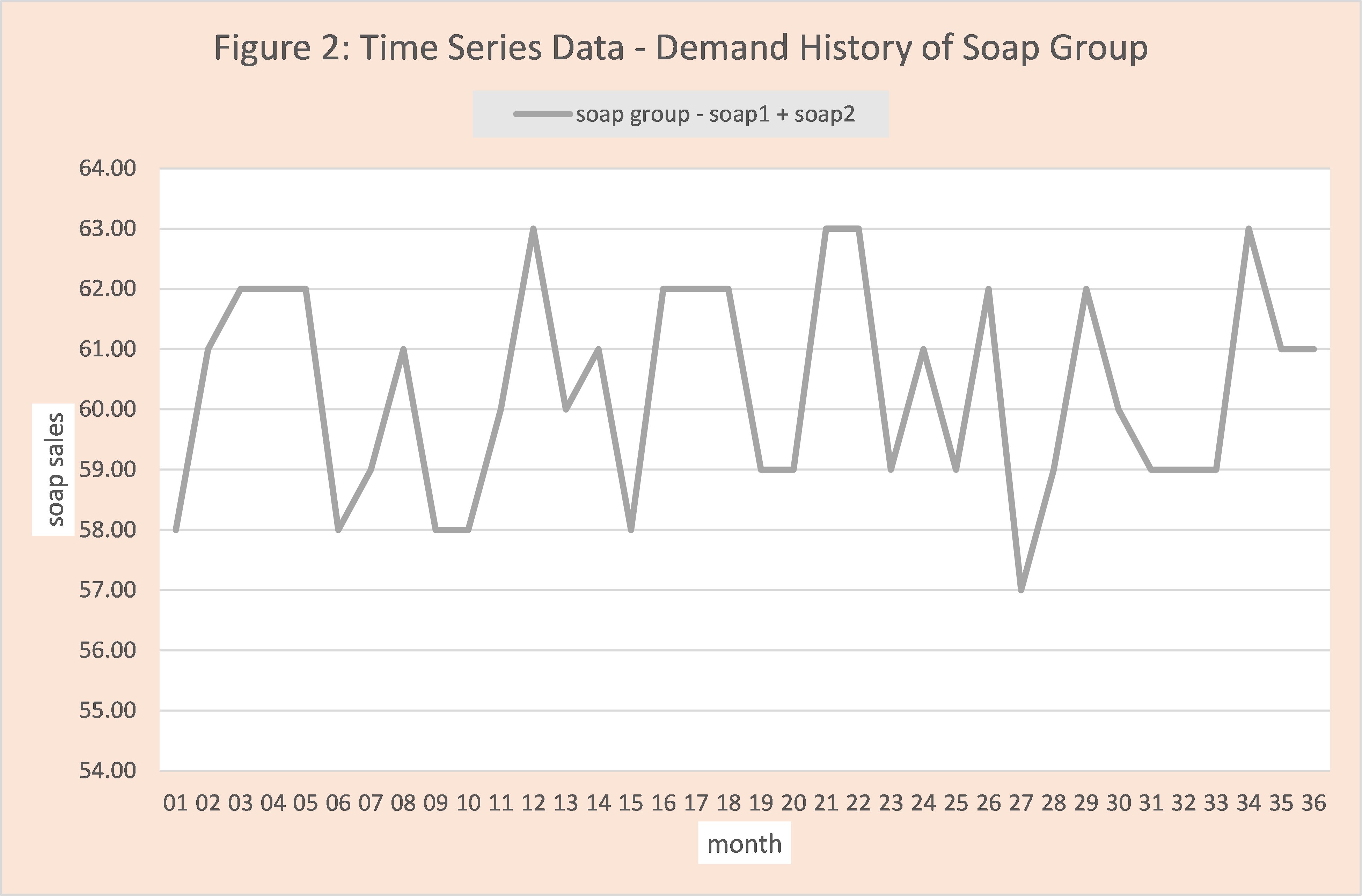
Figure 1 is an example of the type of data we are focused on. We have 36 months of sales history for soap1 and soap2. Figure 2 is the demand history of soap group = soap1 + soap2.
Which type of forecasting
In this blog the focus is “just time series” analysis. In the soap example in figure 1 the only data we must work is the 36 months of sales history for each soap product or SKU. Causal forecasting (could we relate soap sales to an economic or marketing activity) or bottoms up simulation (deterministic or Monte Carlo) is a topic for another time.
How to assess the “forecastability”
Having established what data and which forecasting, we can address the primary question – is my demand forecastable, or how forecastable? There are three primary tasks.
- Is there pattern in the historic data to use and will this pattern continue into the future?
- Do I have the forecasting tools to find and specify the pattern?
- How much “natural variation or uncertainty” is inherent in the demand process?
Tasks 1 and 2 are closely linked. If I don’t have the tools to identify the pattern, there is no way to know if there is a pattern. Consider diagnosing diseases or ailments. Many different ailments present the same. For example, fever is a common symptom of infection from COVID-19 to a cold to a blood infection to cellulitis. When a patient presents with a fever, this triggers further investigation to assess the most likely cause. A second example is swollen feet – possible causes include gout, a bruise, or blocked artery. Arkieva has an advanced three phase strategy to determine if a pattern exists and to specify it.
- It applies artificial intelligence and advanced statistical diagnostic (from first order difference to autocorrelation to non-parametric methods such as run test) to profile or categorize the time series. Categories include, but are not limited to seasonal (cyclical), trend up or down, stationary, intermittent, and not enough data. Figure 1 and 2 has a data set that is stationary. Stationary is defined as random variation around a mean or average value. Fig 3 has umbrella sales history where there is clearly a cyclical or periodic pattern.
- After the profiling is complete, a set of time series forecasting methods is identified to compete to find and specify the profile. This is called the “fit process”. A critical component of this process is the application of optimization methods to find the parameters that optimize the fit – that is minimize the error sum of square of errors (SSE) or sum of the absolute errors (SAE). For example, finding the slope (b1) and intercept (b0) for the best fit linear regression model.
- Since Arkieva has an extensive set of “time series” methods, it then selects the best method based on the user’s choice of metrics – for example MAPE. We will use umbrella sales (Figure 3) to make clear why this important.
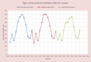
Clearly the umbrella sales had a periodic pattern that repeats yearly. There are many methods that apply to this type of situation, but they have different “skill levels” at capturing the details of the pattern. One common and pretty powerful skill level is seasonality that makes use of concepts from Fourier analysis relying on sine and cosine (a topic for another blog). We will call this FS (Fournier Seasonality). Figure 4 has the best fit (optimized parameters) of FS to the umbrella data set. This is pretty good with average or mean absolute error 3.53.
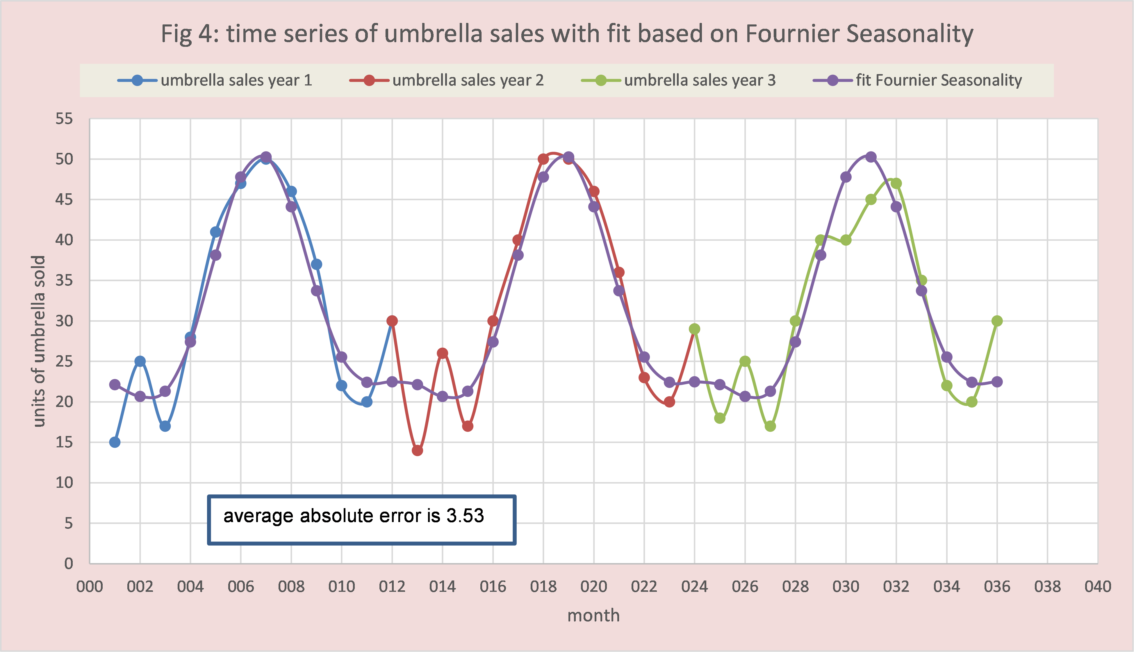
In many forecasting applications, the process would stop here; however, in Arkieva a number of other methods are allowed to compete, including ARIMA. Figure 5 demonstrates ARIMA does a better job at capturing the pattern.

Lesson 1: A critical component of forecastability is the tools you have in your tool kit.
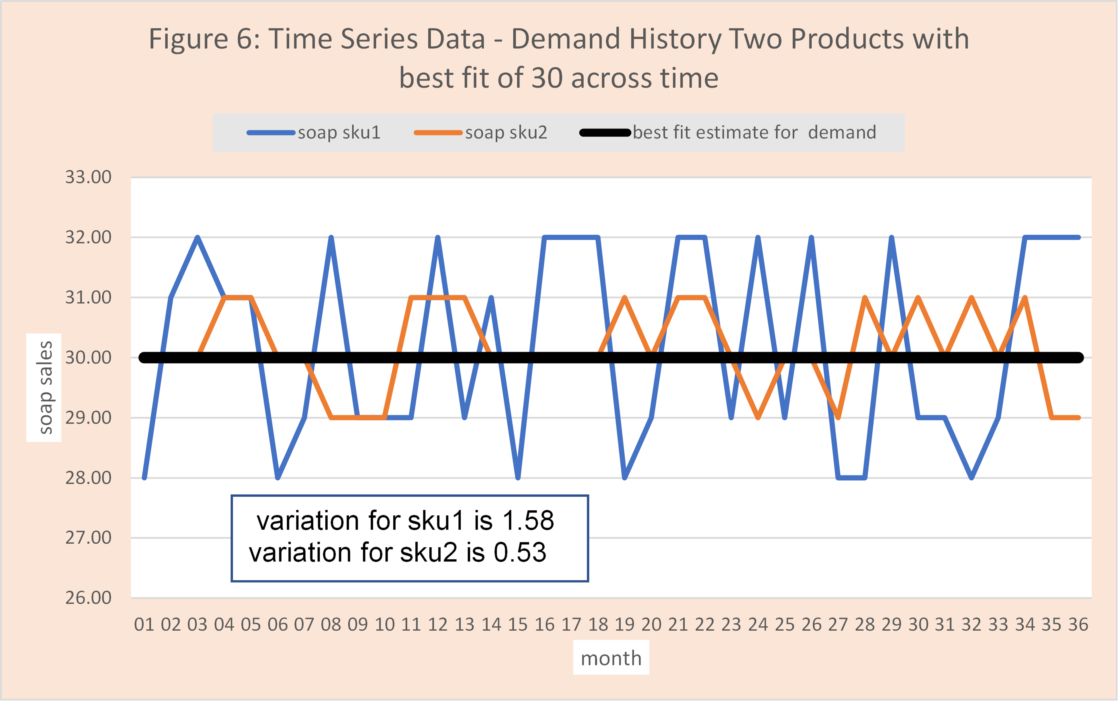
The third task was assessing the inherent variability or uncertainty in the time series data. This cannot be reduced with tools in your forecasting tool bag but is inherent in the process generating the demand. However, without sophisticated tools you cannot determine this is the best you can do. For the two soap demands the best estimate of demand is 30. Figure 6 shows
sku1, sku2, and the stationary estimate of 30. We see sku1 has more variability or uncertainty than sku2. Additionally (separate analysis) the variation is stationary across time.
Interesting observation the rule of thumb is variability is reduced with aggregation. This is not true for our Soap example. A topic for another time.
Lesson 2: The forecastability is limited by the inherent variability in the process generating demand.
Will the Pattern Continue in the Future?
This the million-dollar question and unless you have Merlin on retainer, it is impossible to know. COVID-19 has made this clear. A best-in-class firm uses demand sensing for an early alert to changing conditions. Within the demand estimation process, a fit/predict or train/verify process is a critical component of the Arkieva demand estimation process. An overview of this methodology is provided in Demand Forecasting Analytical Methods: Fit Vs. Predict
Conclusion
One of the top questions in SCM is “is my demand forecastable?” It would be great if there was one simple metric that could be calculated for each time series data set that provided this insight. As in medicine this is not possible. We would not accept our medical team making a diagnosis based on just temperature and blood pressure, we should not accept our provider of demand management to make this assessment simply using co-efficient of variation (COV) and simple least squares fit. As in medicine there are several advanced methods in demand estimation that can handle the complex question of forecastability with a limited amount of workload on the user. Arkieva has deployed these methods in its smart forecasting modules that pulls on expert systems, statistical methods, optimization, and machine learning imbedded in an easy to use software environment.