In a previous blog post, I talked about how a high or low value of Coefficient of Variation (CV) impacts the first or second term of safety stock. My colleague Manjeeth and I decided to put this to the test using real customer data. Here we will discuss our findings.
But first, let us summarize the main points from the above-referenced blog:
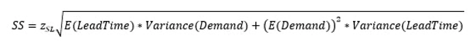
First, remember that CV is calculated as the standard deviation divided by the mean. Further, the formula for safety stock is as follows:
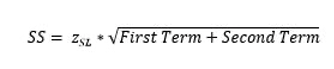
Or as we simplified it:
A high CV implies the first term of the safety stock formula that includes variation of demand becomes important and accounts for a higher percentage of the safety stock. Conversely, a low CV implies that the second term of the safety stock formula which includes the average demand becomes important and accounts for a higher percentage of the safety stock.
We analyzed some data to see if this theoretical inference is backed by data. For this analysis, we used the following classification for CV:
- Low: <= 0.5
- High: More than 0.5
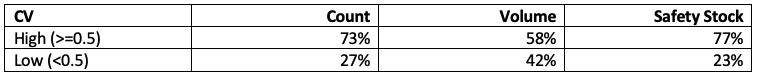
CPG company example
Average Monthly Demand ranged from 1 unit to over 18,000 per month.
CV ranged from 0.42 to 3.0.
The average lead time was 7 days.
The total Safety stock is 862K units. Of this, 88% comes from the first term and 12% comes from the second term.
The table below summarizes the results by high/low CV.
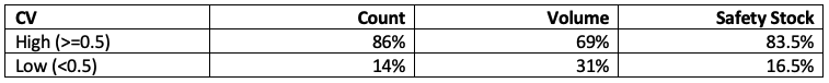
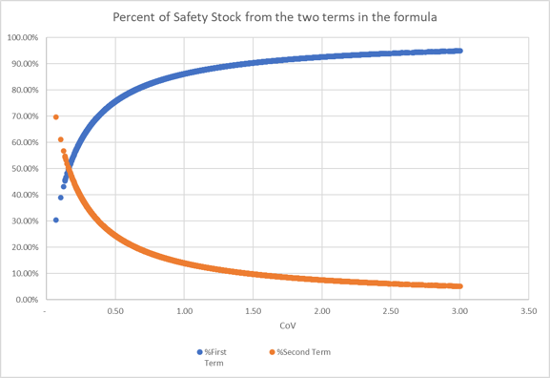
The graph below shows the results of the data analysis for this data set.
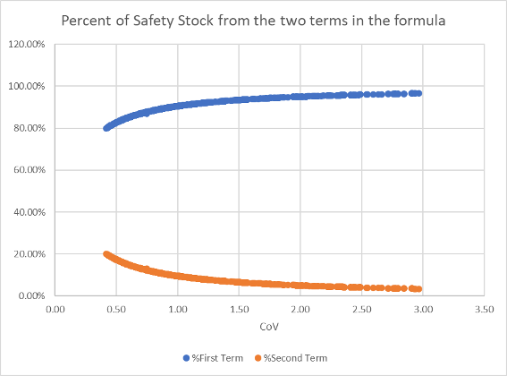
Looking at the results, when the CV is low, the first term accounts for the majority (>80+%) of the safety stock in all cases. Further, as the CV increases, the percent of the safety stock from the first term increases.
Industrial Parts Example
Average Monthly Demand ranged from 4 units to over 6.5M per month.
CV ranged from 0.07 to 3.
The average lead time was 21 days.
Total Safety Stock is 201M units. Of this, 81% comes from the first term and 19% comes from the second term.
The table below summarizes the results by high/low CV.
The graph below shows the results of the data analysis for this data set.
Chemical Industry Example
Average Monthly Demand ranges from 10 units to over 2.5M per month.
CV ranges from 0.09 to 4.
The average lead time was 20 days.
Total Safety Stock is 1,947M units. Of this, 67% comes from the first term and 33% comes from the second term.
The table below summarizes the results by high/low CV.
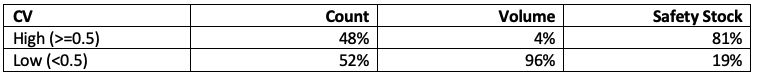
This dataset is different from the other two in that a bigger portion of the data is low CV.
The graph below shows the results of the data analysis for this data set.
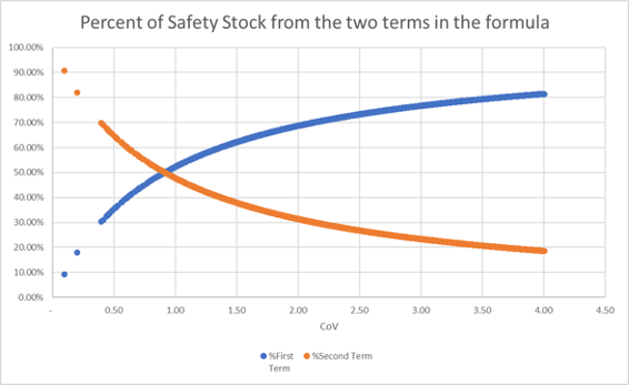
As can be seen from all three data sets:
- Most of the safety stock comes from the first term.
- This is true even in the case of the third dataset where most of the data is low CV.
- An increase in CV creates an increase in the safety stock coming from the first term of the safety stock formula.
- For very high CV values, the 2nd term contributes very little to the overall safety stock.
So, what are the practical implications of this?
As demand is an external variable (in that outside forces/factors determine what the demand would be), there is not much that can be done about the mean demand. Some businesses might have avenues like negotiating different contracts with customers or being able to do demand shaping to smooth out the demand.
However, demand variance can be decreased if one has a good forecasting process. By good, we mean that the forecast generated does a better job of forecasting than the mean. Here is a practical (not statistical) way to think about it. In the calculation of the safety stock, one uses mean demand and calculates the variance from it. If through a forecasting process, one could generate a forecast that came closer than the mean in predicting the future, then one could substitute the demand variance with the variance of the forecast error. This could impact the first term very substantially, depending on the accuracy of said forecast.
The effects were as follows in the three data sets we experimented with:
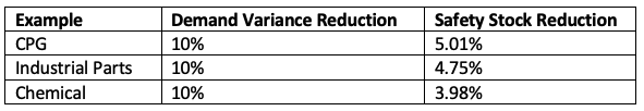
Conclusion 1: A 1% decrease in demand variance helps save 0.4% to 0.5% from safety stocks. If a company has $100M worth of inventory, and 25M of those is from safety stocks, then a 10% reduction in demand variance (typically through better forecasting) will take out about $1M from inventory. Given the cost of a typical demand planning project, that is a very good ROI.
Now let us look at the other two recommendations from the above-referenced blog.
- If your product has a high CV or high forecast error, work on reducing the mean lead time.
- For example, you might be sourcing the product from overseas and may consider finding a local supplier.
- If your product has a low CV or low forecast error, work on eliminating the variation in the supply of the product.
- This could mean working on processes, getting more reliable and higher-quality suppliers, etc.
Let us simulate these changes in the three data sets.
Focusing first on the high variation items, let us evaluate the net changes when one reduces the lead time for combinations with High CV.
If we focus only on the high CV part of the data, the safety stock reduction can be summarized as follows:
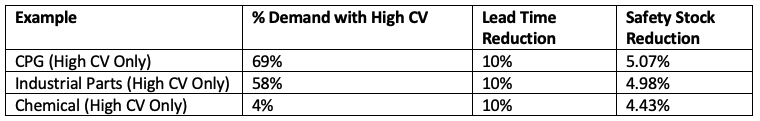
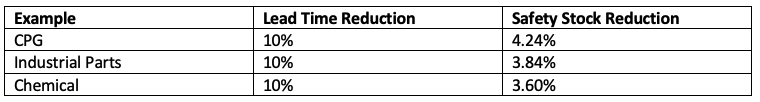
Conclusion 2: A 1% decrease in mean lead time can help save 0.3% to 0.4% from safety stocks. This number depends on how much of the data has a high CV. In the example company above with $25M in safety stocks, this could mean a savings of $750K. Changing mean lead time could be done in two ways: Finding suppliers that are close by and/or using faster transportation modes. Both have extra costs associated with them, so they need to be weighed appropriately.
Next, let us look at items with Low CV. The suggestion here was to reduce the lead time variation. The table below shows the result.
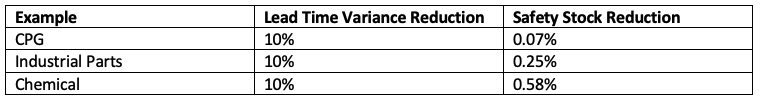
If we focus only on the low CV part of the data, the safety stock reduction can be summarized as follows: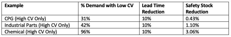
Conclusion 3: A 1% decrease in lead time variance can save 0.05% to 0.1% from safety stocks. In the example company above with $25M in safety stocks, this could mean a savings of $250K. This is obviously less of an impact compared to the change in mean lead time. In fact, the final savings depend on the proportion of the demand that shows low variation. These days, for most businesses, the demand is increasingly variable. The variation in the lead time could be impacted by negotiating better terms with the suppliers, improving production and scheduling processes, etc.
So, let us summarize the results here.
- Most of the safety stock comes from the first term in the formula.
- Most of the safety stock sits on High CV combinations.
- Reducing demand variance via an improved forecasting process can significantly reduce the investment in safety stocks. This implies that an investment in a better forecast will have a good ROI.
- Reducing lead time for highly variable items can significantly reduce the investment in safety stocks for that portion of the supply chain. This method can be employed where a large proportion of the demand is highly variable.
- Reducing the variation of the lead time can also reduce the investment in safety stocks for that portion of the supply chain, albeit less than the above two changes. This method can be deployed if a large proportion of the demand has low variation. Unfortunately, this seems to be a rarity these days.
- The best use of money (highest ROI) would be to try and decrease demand variance (likely through better forecasting) and mean lead time.
Enjoyed this post? Subscribe or follow Arkieva on Linkedin, Twitter, and Facebook for blog updates.

About the Author: Sujit Singh
As COO of Arkieva, Sujit manages the day-to-day operations at Arkieva such as software implementations and customer relationships. He is a recognized subject matter expert in forecasting, S&OP, and inventory optimization. Sujit received a Bachelor of Technology degree in Civil Engineering from the Indian Institute of Technology, Kanpur, and an M.S. in Transportation Engineering from the University of Massachusetts. Throughout the day don’t be surprised if you find him practicing his cricket technique before a meeting.

About the Author: Manjeeth Vijayan
Manjeeth A Vijayan is a Senior Consultant at Arkieva, India. He is responsible for analyzing client’s supply chain processes, configuring and implementing Arkieva software, thereby, helping clients improve efficiencies in their supply chain planning. He received a Bachelor Of Technology degree and went on to earn his masters in Industrial Engineering from the National Institute Of Industrial Engineering, India. He is also an APICS certified CPIM (Master Planning of Resources) certificate holder. Other than supply chain, traveling and hiking excite him these days.