January 29 is National Puzzle Day, and in celebration, we’ve created a fun blog that details how to solve Sudoku using artificial intelligence (AI).

Introduction

Before Wordle, the Sudoku puzzle was the rage and it is still very popular. In recent years, the use of optimization methods to solve the puzzle has been a dominant theme. See “Solving Sudoku Puzzle Using Optimization in Arkieva”.

In current times, the use of AI is focused on machine learning which encompasses a wide range of methods from lasso regression to reinforcement learning. The use of AI has reemerged to tackle complex scheduling challenges. One method, search with backtracking, is commonly used and is perfect for Sudoku.

This blog will provide a detailed description on how to use this method to solve Sudoku. As it turns out, “backtracking” can be found inside optimization and machine learning engines and is a cornerstone of the advanced heuristics Arkieva uses for scheduling. The algorithm is implemented in an “Array Programming Language, ” a function-orientated programming language that handles a rich set of array structures.

Basics of Sudoku

From Wikipedia: Sudoku is a logic-based, combinatorial number-placement puzzle. The objective is to fill a 9×9 grid with digits so that each column, each row, and each of the nine 3×3 sub-grids that compose the grid (also called “boxes”, “blocks”, “regions”, or “sub-squares”) contains all of the digits from 1 to 9. The puzzle setter provides a partially completed grid, which typically has a unique solution. Completed puzzles are always a type of Latin square with an additional constraint on the contents of individual regions. For example, the same single integer may not appear twice in the same 9×9 playing board row or column or in any of the nine 3×3 subregions of the 9×9 playing board.

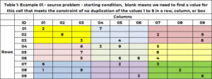
Table 1 has an example problem. There are 9 rows and 9 columns for a total of 81 cells. Each is permitted to have one and only one of nine integers between 1 and 9.  In the starting solution, a cell either has a single value – which fixes the value in this cell to that value, or the cell is blank, indicating we need to find a value for this cell. The cell (1,1) has the value 2 and cell (6,5) has the value 6. Cell (1,2) and cell (2,3) are blank, and the algorithm will find a value for these cells.

The Complication

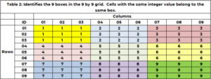
In addition to belonging to one and only one row and column, a cell belongs to one and only 1 box. There are 9 boxes, and they are indicated by color in Table 1. Table 2 uses a unique integer between 1 and 9 to identify each box or grid. The cells with a row value of (1, 2 or 3) and column value of (1, 2 or 3) belong to box 1. Box 6 is row values of (4, 5, 6) and column values (7, 8, 9). The box id is determined by the formula BOX_ID = {3x(floor((ROW_ID-1) /3)} + ceiling (COL_ID/3).  For the cell (5,7), 6 = 3x(floor(5-1))/3) + ceiling (8/3)= 3×1 + 3 = 3+3.

The Heart of the Puzzle

To find one integer value between 1 and 9 for each unknown cell such that the integers 1 to 9 are used once and only once for each column, each row, and each box.

Let’s look at cell (1,3) which is blank. Row 1 already has the values 2 and 7. These are not allowed in this cell. Column 3 already has the values 3, 5,6, 7,9. These are not allowed. Box 1 (yellow) has the values 2, 3 and 8. These are not allowed. The following values are not allowed (2,7); (3, 5, 6, 7, 9); (2, 3, 8). The unique values not allowed are (2, 3, 5, 6, 7, 8, 9). The only candidate values are (1,4).

A solution approach would be to temporarily assign 1 to cell (1,3) and then try to find candidate values for another cell.

A Backtracking Solution: Starting Components

Array Structure

The starting place is to decide on an array structure to store the source problem and support the search. Table 3 has this array structure. Column 1 is a unique integer id for each cell. The values range from 1 to 81. Column 2 is the row ID of the cell. Column 3 is the column ID of the cell. Column 4 is the box id. Column 5 is the value in the cell. Observe a cell without a value is given the value zero instead of blank or null. This keeps this an “integer only array” – far superior for performance.

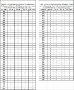
In APL, this array would be stored in a 2-dimensional array where the shape is 81 by 5. Assume the elements of Table 3 are stored in the variable MAT.  Example functions are:

The command MAT[1 2 3;]grabs the first 3 rows of MAT
1 1 1 1 2
2 1 2 1 0
3 1 3 1 0
MAT[1 2 3; 4 5] secures rows 1, 2, 3 and just columns 4 and 5
1 2
1 0
1 0
(MAT[;5]=0)/MAT[;1] finds all cells that need a value.

INSERT TABLE 3

Sanity Check: Duplicates

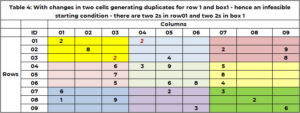
Before starting the search, it is critical to sanity check!  That is the starting solution feasible. Feasible for Sudoku, is there are now duplicates in any row, column, or box. The current starting solution, for example, 1 is feasible. Table 4 has an example where the starting solution has duplicates. Row 1 has two value 2. Area 1 has two value 2. The function “SANITY_DUPE” handles this logic.

Sanity Check: Options for Cells without Values

A very helpful piece of information would be all of the possible values for a cell without a value. If there are no candidates, then this puzzle is not solvable. A cell cannot take on a value that is already claimed by its neighbor. Using Table 1 for Cell (1,3,’1’ – this last 1 is the boxid), its neighbors are row 1, column 3, and box 1. Row 1 has the values (2,7); column 3 has the values (3,5,6,7,9); box 1 has the values (2,3,8). Cell (1,3.1) cannot take the following values (2,3,5,6,7,8,9). The only options for cell (1,3,1) are (1,4). For cell (4,1,2) the values 1, 2, 3, 5, 6, 7, 9 are already used in row 4, column 1, and/or box 4. The only candidate values are (4,8). The unction “SANITY_CAND” handles this logic.

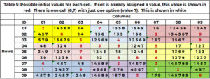
Table 5 shows the candidates, for example, 1 at the start of the search process. If a cell has already been assigned a value in the starting conditions (Table 1), then this value is repeated and shown in red. If a cell that needs a value has only one option, this is shown in white. Cell (8,7,9) has the single value 7 in white. (2,5,8,4,3) are claimed by neighbor column 7. (1, 2, 9) by row 8. (3,2,6) by box 9. Only the value 7 is unclaimed.

Sanity Check: Looking for Conflicts

The information identifying all options for cells that need a value (posted in Table 4), enables us to identify a conflict before starting the search process. A conflict occurs when two cells that need a value have only one candidate, the candidate value is the same, and the two cells are neighbors. From Table 4 we know the only cell that needs a value and has only one candidate is cell (8,7,9). For example 1, there is no conflict.

What would be a conflict?  If the only possible value for cell (3,7,3) was 7 (instead of 1, 6, 7), then there is a conflict. Cell (8,7) and cell (3,7) are neighbors – the same column. However, if the only possible value for cell (4,9,2) was 7 (instead of 1, 2, 7) this would not be a conflict. These cells are not neighbors.

Sanity Check Summary

1. If there are duplicates, the starting solution is not feasible.
2. If a cell that needs a value, does not have any candidates, then there is no possible solution to this puzzle. The list of candidate values for each cell can be used to reduce the search space – both for backtracking and optimization.
3. The ability to find conflicts identifies the puzzle is not feasible – has no solution – without a search process. Additionally, it identifies the “problem cells”.

A Backtracking Solution: Search Process

With core data structures and sanity checking in place, we turn our attention to the search process. The recurring theme is again, getting data structures in place to support search.

Tracking the Search

The array Tracker keeps track of the assignments made

1. Col 1 is the counter
2. Col 2 is the number of options available to assign to this cell
   • 1 means 1 option available, 2 means two options, etc.
   • 0 means – no option available or resetting to 0 (no assigned value) and backtracking
3. Col 3 is the cell assigned a value index number (1 to 81)
4. Col 4 is the value assigned to the cell in track history
   • A value of 9999 means this cell was when the dead end was found
   • The value of an integer between 1 and 9 inclusive, is the assigned value to this cell at this point in the search process.
   • A value of 0 means this cell needs an assignment

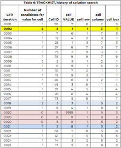
The tracker array is used to support the search process. The array TRACKHIST has the same structure as the tracker but keeps the history of the entire search process. Table 6 has part of TRACKHIST for example 1. It is explained in more detail in a later section.

Additionally, the array PAV (a vector of a vector), keeps track of Previously Assigned Values to this cell. This ensures we don’t revisit a failed solution – similar to what is done in TABU.

There is an optional log process where the search process writes out each step.

Starting the Search

With bookkeeping and sanity checking done, we can now start the search process. The steps are:

1. Are there any cells left that need a value? – if no, then we are done.
2. For each cell that needs a value, find all candidate options for each cell. Table 4 has these values at the start of the solution process. At each iteration, this is updated to accommodate values assigned to cells.
3. Evaluate the options in this order.
   • If a cell has ZERO options, then institute backtracking
   • Find all the cells with one option, select one of these cells, make this assignment,
     1. and update the tracking table, the current solution, and PAV.
   • If all the cells have more than one option, then select one cell and one value, and update
     1. and update the tracking table, the current solution, and PAV

We will use Table 6 which is part of the history of the solution process (called TRACKHIST) to illustrate each step.

In the first iteration (CTR=1), cell 70 (row 8, col 7, box 9) is selected to be assigned a value. There is just candidate (7), and this value is assigned to cell 70. Additionally, the value 7 is added to the vector of previously assigned values (PAV) for cell 70.

In the second iteration cell 30 is assigned the value 1. This cell had two candidate values. The smallest candidate value is assigned to the cell (just an arbitrary rule to make the logic easy to follow).

The process of identifying a cell that needs a value and assigning a value works fine until iteration (CTR) 20. Cell 9 needs value, but the number of candidates is ZERO. There are two options:

• There is no solution to this puzzle.
• We undo (backtrack) some of the assignments and take another path.

We looked for the cell assignment closest to this, where there was more than one option. In this example, this occurred at iteration 18, where cell 5 is assigned the value 3, but there were two candidate values for cell 5 – values 3 and 8.

Between cell 5 (CTR = 18) and cell 9 (CTR = 20), cell 8 is assigned the value 4 (CTR=19). We put cells 8 and 5 back on the “need a value” list. This is captured in the second and third CTR=20 entries, where the value is set to 0. The value 3 is kept in the PAV vector for cell 5. That is the search engine cannot assign the value 3 to cell 5.

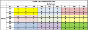
The search engine starts up again to identify a value for cell 5 (with 3 no longer an option) and assigns the value 8 to cell 5 (CTR=21).  It continues until all cells have a value or there is a cell with no option and there is no backtracking path. The solution is posted in Table 7.

Observe, where there is more than one candidate for a cell, this is a chance for parallel processing.

Comparison with MILP Optimization Solution

At the surface level, the representation of the Sudoku puzzle is dramatically different. The AI approach uses integers and by any measure is a tighter and more intuitive representation. Additionally, the sanity checkers provide helpful information to make a stronger formulation.  The MILP representation is endless binaries (0/1). However, the binaries are powerful representations given the strength of modern MILP solvers.

However, internally, the MILP solver does not keep the binaries but uses a sparse array method to eliminate storing all of the zeros. Additionally, the algorithms to solve binaries do not emerge until the 1980s and 1990s. The 1983 paper by Crowder, Johnson, and Padberg reports on one of the first practical solutions of optimization with binaries. They note the importance of clever preprocessing and branch and bound methods as critical to a successful solution.

The recent explosion of the use of constraint programming and software such as local solver has made clear the importance of using AI methods with the original optimization methods such as linear programming and least squares.