Summary
In previous blogs, we discussed reasons to make the technology investment. In future blogs, we will continue this discussion, where a key topic will be “write once and read never” for complex Excel worksheets. This blog is focused on protecting your investment. The example focuses on the difference between demand variability and prediction variability and its impact on inventory and operational effectiveness. Demand variability is the variation in demand across time. Prediction variability is the variability within a time period. Figure 2 illustrates the difference. Prediction variability requires a prediction interval or probabilistic forecast to augment the point forecast. If your consultant gets this wrong – there are troubles ahead. The blog is loosely based on a real situation from the trenches. The blog also touches on the importance of central planning.
Introduction
In previous blogs, we discussed reasons to make the technology investment. In future blogs, we will continue this discussion, where a key topic will be “write once and read never” for complex Excel worksheets. The examples below are two lines of “Excel code” that I wrote. The only way I could make sure they were giving the correct results was to code in a “regular language” and compare the results.
- “=IF(need!F13=0,IF(delta!F13>0,$E$359,$E$356),IF(delta!F13>0,$E$357,IF(delta!F13<0,$E$354,$E$355)))”
- “=COUNTIF(use!H$14:use!H$259,$D14)”
This blog is focused on protecting your investment. The example involves demand variability versus prediction variability and its impact on inventory policy and operational efficiencies. It is loosely based on a real situation from the trenches.
The Scene of the Crime
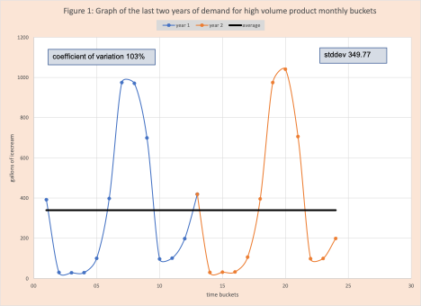
The firm (IC) sells ice cream year-round, much of which it produces locally. At a holiday party, the CEO chatted with the marketing person from a supply chain management firm (CMF) who was certain her firm could optimize the ice cream inventory. In early February, a recently APICS certified consultant visited the firm, briefly chatted with the CDO (chief of daily operations), and then worked directly with the senior inventory planner. The consultant asked for two years of demand data in monthly buckets for one of the most popular (high volume) flavors. Table 1 displays this data. Figure 1 is a graph of this data.
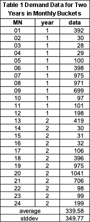
The consultant calculated the average, standard deviation, and coefficient of variation (COV) of the demand history. With a COV value of 103%, she declared the demand is highly variable which will require substantial safety stock to protect against lost sales due to lack of ice cream. The consultant used the standard formula that she proudly stated was from the APICs text.
The planner was puzzled by two items:
- The new upper bounds were going to require more production then are currently available.
- The new upper bounds to protect against a shortage were much higher than the one they had been using with some success, shown in table 2.

The consultant with the inventory planner brought the results back to the CDO with the questions not really resolved. The CDO knew the CEO was anxious to bring best in class SCM expertise and software to bear on their operations – and be able to go the next holiday party and tell folks how machine learning had improved operational efficiencies. To do this a contract needed to be in place by early March.
What to do?
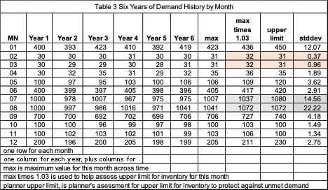
The CDO suggested the planner visit the local business school and asked to chat with a professor with some applied experience and a disciple of Gene Woolsey. The professor met with the planner and then referred him to an “aging wing tip warrior” (AWTW) who could often be found at the playground with his grandchildren. He found the person and posed the question. They met two days later in secret. The planner showed the AWTW the numbers they used to bound risk (table 2). AWTW then asked how they arrived at these numbers – something the planner did not expect. The planner explained they looked at demand across the same month for the last six years (Table 3), found the maximum for each month across years, used a multiplier of 1.03, and then made some manual adjustments based on their feel for uncertainty and where the month was within the pretty consistent yearly pattern referred to as two scoops. AWTW asked for examples of the adjustments. The planner provided two.
- For months 7, 8, and 9 the planner used a higher fudge factor for month 7 (from 1037 to 1080) then no fudge for month 8. If there was unused ice cream in month 7, it could be used in month 8 since the ice cream was made each week and had a shelf life of 4 weeks, with a preferred sell within 2 weeks.
- For months 2 and 3, he used no fudge factor since there was very limited variability.
-
- The AWTW then added the standard deviation calculation to the planner’s table and showed them how the low standard deviation values for these months backed up their instincts about low variability.
- AWTW pointed out the standard deviation for month 8 was much higher than in month 7. Perhaps that depended on when the first cool spell came in August.
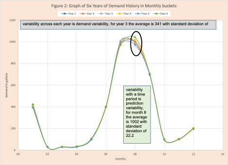
AWTW then created a graph of the demand history data the planner was using to create a visual (Figure 2) that made clear demand variability across time was the dominant factor, while variability within a time bucket was small. Variability within a time period was often called prediction variability.
The planner then posed the difficult question – what steps to take next?
AWTW suggested the planner take the cleaned-up example in excel with the multicolored graph back to the consultant with notes from their discussion and a concept called community intelligence. Tell the consultant they had chatted with the university professor who was an APICs certified black belt and they suggested splitting variability into demand and prediction variability which was the latest concept from data science.
The last question posed by AWTW was how the firm was making production start decisions to match assets with demand to meet shelve life requirements, preferred sell-by date, balance production where there are different productive capacity across time, and provide folks time to ski or travel south for a bit of the winter. He noted this was a critical need, but a topic for another time. It was an area called central planning.
Conclusion
Clearly once a person sees Figure 2, it is obvious the dominant feature is very predictable, but sizeable variation across time (demand variability) and limited variation within a month (prediction variability). Therefore, the prediction error for a monthly bucket is small. It is not uncommon, that once a person starts down one track, it is not always easy to shift gears. This is what Gary Sullivan referred to as the danger of painting by numbers.
It is important to note for ice cream the variation day to day or week to week can be substantial (weather events, road repair, etc.) and this variation is lost with monthly data. These variations require a responsive demand-supply network with tools to support decision tiers three and four.
Enjoyed this post? Subscribe or follow Arkieva on Linkedin, Twitter, and Facebook for blog updates.