Summary
The current mantra that dominates business forecasting conversations is even the slightest improvement in forecast accuracy drives huge improvements in a firm’s performance, dwarfing improvements in other aspects of supply chain management. In fact, there is often very limited value to the firm for three reasons: unanchored value, mirage or illusion of random variation, and a narrow metric of improvement. Insights from professionally applied statisticians can help a firm distinguish between real value and phantom values. These insights are: (a) is it worth the effort, (b) overfitting, and (c) random variation. These will be illustrated using an example where the bulk of the technical material is pulled from chapters 1 and 2 in the classic text on Applied Linear Statistical Models by Neter and Wasserman. The real impact of demand estimates can only be determined with a central plan and community intelligence.
Introduction
The common mantra in forecasting or demand estimation is a 3% increase in forecast accuracy generates huge improvements in business performance dwarfing improvements in other aspects of supply chain management. In fact, there is often very limited or no value to the firm for three reasons: unanchored, mirage or illusion, and a narrow metric of improvement. Unanchored refers to the value of the improvement not also being a function of the current level of forecast accuracy. For example, a 3% increase from a base of 90% accuracy has the same value as a 3% increase from a base of 30% accuracy – unlikely. Mirage refers to the well-known concept that the “improvement” is simply the “luck of the draw” (random variation). The metric of improvement is typically narrow in scope – using the lengthy portion of the far past to estimate a few time periods of the near past. With the ever-growing interest in the application of computational methods to estimate demand, and diverse technical groups (data science, machine learning, business statistics, supply chain experts, etc.) participating in this area, this blog covers critical insights from professionally applied statisticians who have learned early in their educational process – is it worth the effort, overfitting, and random variation. These will be illustrated using the following example where the bulk of the technical material is pulled from chapters 1 and 2 in the classic text on Applied Linear Statistical Models by Neter and Wasserman.
Example 1
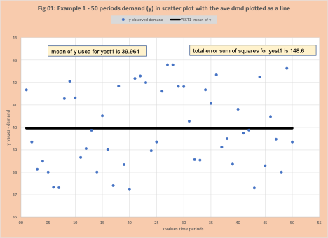
Our example is 50 periods of demand that is plotted in Figure 1 as a scatter plot. Table 1 has the first 10 periods of demand. Column 2 is the demand for this period. Column 3 is YEST1 where the average demand across the 50 time periods (39.964) is used as an estimated value for Y (demand). In figure 1 this is plotted as the solid line. Why the use of the mean of y?


An early lesson in statistics is to start with the average as the estimate of demand and assess how well this works. The metric is the “error squared”. In table 1 time period 1, y is 41.672, yest1 is 39.964, their difference is 1.708 (=41.672 – 39.964) in column 4, and the square of the error is 2.917 (=1.7082) in column 5. The error is squared to eliminate the negative sign (see Victory of Least Squares to understand why squaring was used). The quality of the estimate is the sum of the squared errors (SSE), which is 148.613. All other methods to estimate demand are compared to the “mean of y” to determine if they are worth the effort.
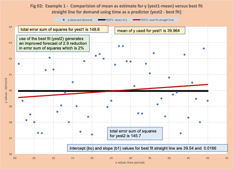
How might we improve our forecast? We find the best fit straight line between the actual demand (y) versus the time period (x). The intercept (b0) is 39.54 and the slope (b1) is 0.0166. This estimate is called EST2 (shown in column 6). This line is displayed in figure 2. The Sum of Squared Errors for EST2 is calculated in the same fashion as with EST1. For the first time period, YEST2 is 39.557 (column 6). ERR2 is 2.115 (=41.672-39.557) in column 7, and the squared error is 4.475 (=2.1152) in column 8. The total is 145.7.

Is it worth the effort?
SSE1 (SSE for YEST1 – the mean) is 148.6. SSE2 (SSE for YEST2 – best fit line) is 145.7. This is a “forecast improvement of 2.9 units which is about 2%. Certainly not large, but still an improvement. The traditional business forecasting mantra is that every little bit helps, and we would select YEST2 as the best method to estimate demand and base our business decisions on these numbers.
A professional statistics perspective is to ask the question – Is it worth the effort? The extra effort is the use of time period to help estimate demand and this can and does improve the quality of the estimate simply because it exists. For example, if we had a second variable to help estimate demand called X2, where X2 is the square root of the time period, this creates YEST3 (best fit on X1 (time period) and X2 (square root of time period). This generates a slightly better estimate based on SSE. SSE3 is 142.731, about 3 units better than SSE2. In fact, the improvement has no basis in reality, it is just a function of adding X2. This is referred to as overfitting.
Does it matter from a business perspective? YES! Each forecasting method carries a different insight into the demand pattern.
- YEST1 says the demand is steady across time, with random variation from a mean value.
- YEST2 says the demand shows a very slight, but steady growth.
This is a substantial impact across time in terms of production capacity, purchasing, and setting financial targets.
The Mirage or Illusion – Random Variation
We are still faced with the issue of which method to use. Does EST2 provide a better estimate in terms of lower SSE? The business statistician and data science experts argue EST2 is the best to use. Everyone knows linear regression is reliable and we should make use of all of the data we have.
However, the professional statistician points that in fact there is NO slow upward trend, this low slope is simply from random variation. In this case, since I created the data set using a Monte Carlo simulation, this is correct. The core of the simulation’s demand is based on a steady demand of 40 per time period with a uniform random variation for each period.
Understand the Business Impact
The purpose of any model or analysis effort is insight. In this case, for this product, the best information we have is steady demand with a random variation or slow growth with random variation. The business question is what the impact on the business is and how does the business best position itself to respond to emerging events. This requires the use of central planning.
Conclusion
The current mantra that dominates business forecasting conversations is even the slightest improvement in forecast accuracy drives huge improvements in a firm’s performance. This drives the application of methodologies that simply provide the illusion of a better forecast where “better” is a narrow measure. Best in class applied statisticians are well trained to watch for this mirage and their potential dangers for a firm. In this blog, we have illustrated through an example of these potential pitfalls (unanchored, random variation, and narrow metrics) and potential negative impact on a firm. The addition of any arbitrary factor to help estimate demand, by definition, reduces the error sum of squares. Random variation can generate the illusion of a slow increase when in fact demand is steady. Firms that fail to heed these insights do so at their own peril.


