Missed the beginning of the series? Catch up on part 1 and part 2.
In this series of blog posts, we have been talking about Jane who is in the role of inventory planner at her company. As part of the journey, she learned about safety stocks and set them up using the period coverage method. Then, she fine-tuned the period coverage method based on the lead time and the coefficient of variation from the supplier. Still dissatisfied with the results of her safety stock calculations, she decided to get some help from a consultant.
When in Doubt, Ask an Expert
Kate, the consultant, had years of experience with safety stock levels and decided to take a coach-like approach with Jane. She confirmed that lead time and demand variability were both important when calculating safety stocks, however, she wanted to expand on these concepts. She started her coaching on the concept of lead times and their impact on effective inventory management.
First, Kate pointed out why the supply lead time was important to ensure the new supply arrived exactly after the lead time had passed. So, if the lead time was 7 days, then ordering today would mean the product would arrive 7 days from today. Also, as far as variability in demand is concerned, one would need to worry about this variability over the length of the lead time. As in, customer demand could be more than the expected amount on all the days during the lead time.
Kate advised Jane to only consider the observed lead time and not the lead time mentioned in agreements or contracts. She explained that the lead time in contracts or the ERP system may not represent the facts on the ground.
Next, Kate pointed out that if the demand was completely steady, one would not need any safety stock. One would order exactly what one needs and receive that amount when the lead time had passed. Kate summarized it thus: No variation, no uncertainty = 100% predictability = no safety stocks (and that it never happens).
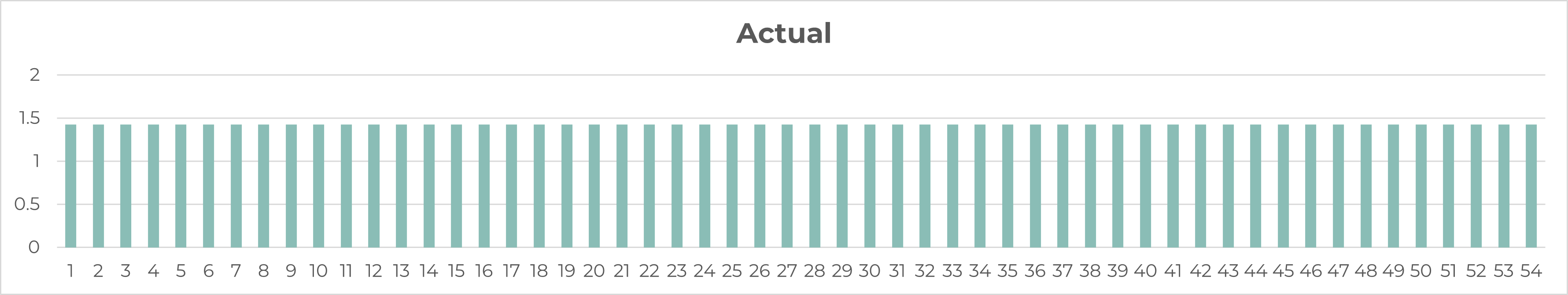
Figure 1
Click to enlarge
Kate suggested using standard deviation as the measure of variability. In Figure 1 above, the average is 1.43, and the standard deviation is 0.
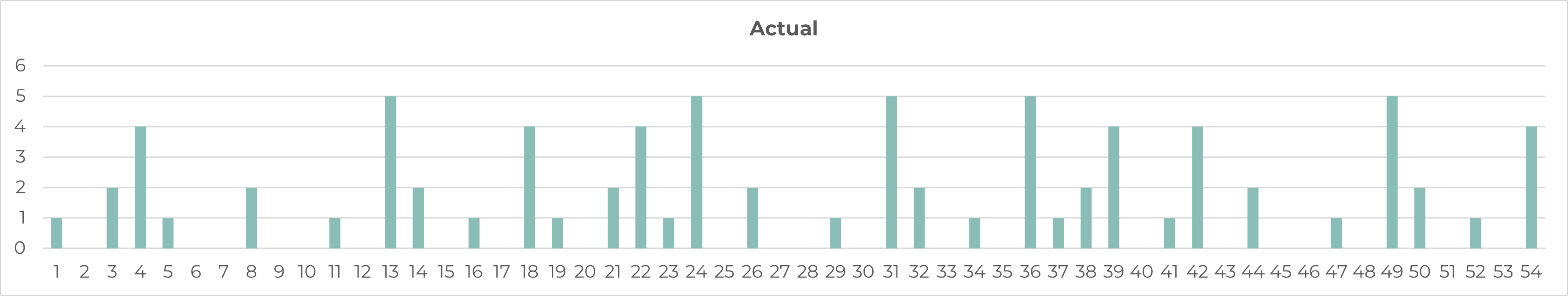
However, if the demand was variable, then one would need to worry about the possibility of the demand being higher than expected. A higher-than-expected demand could result in the inability to supply products to the customer. In the example below, the average is the same as the example above (1.43), but the standard deviation is 1.70. The standard deviation is more than the mean, implying a very variable demand at the daily level.
Figure 2
Click to enlarge
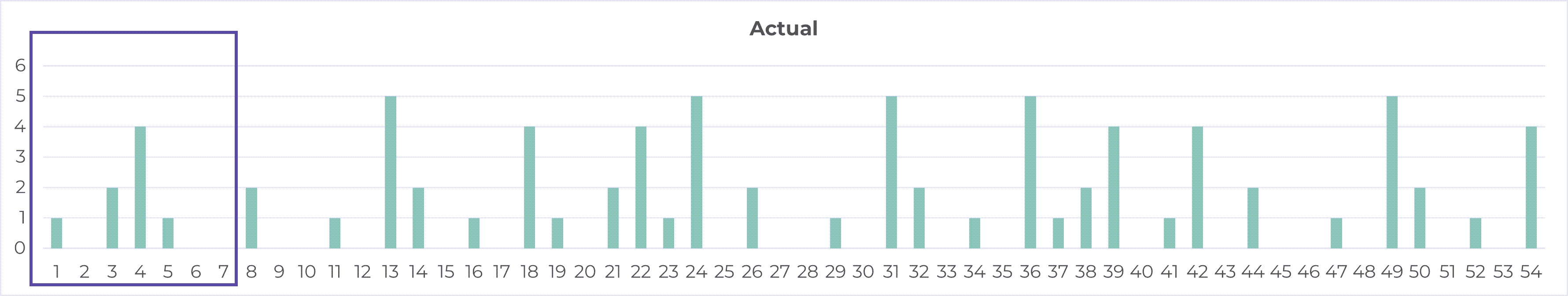
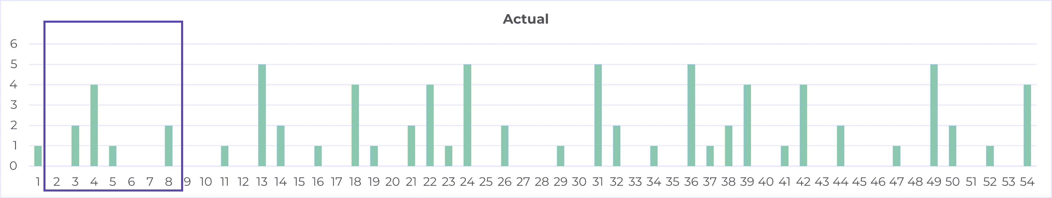
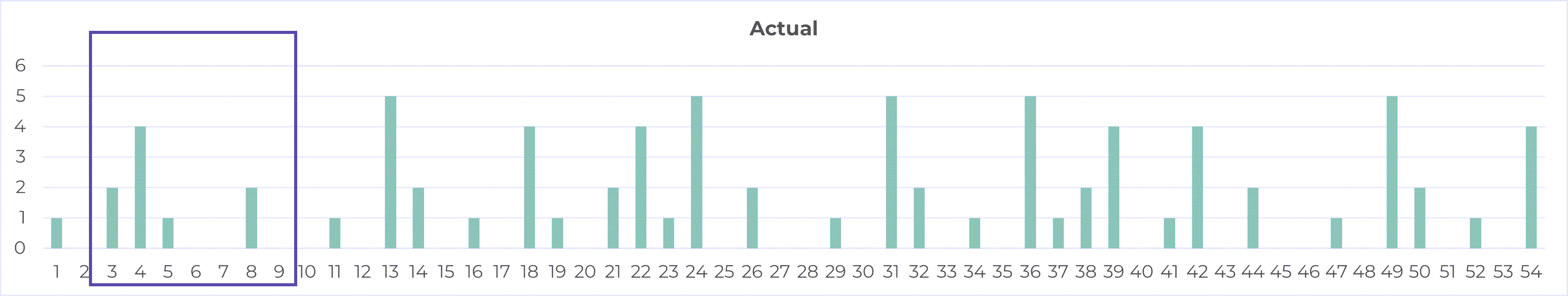
Kate suggested that this might be too conservative an approach if the lead time was more than 1 day. Typically, high-demand days might be balanced with low-demand days and a more stable picture could emerge over the length of the lead time. And therefore, Kate advised looking at the demand in time buckets of size equal to the lead time. With an example lead time of 7 days, one needs to look at the demand through a lens that was 7 days wide (Figures 3 through 9).
Figure 3
Click to enlarge
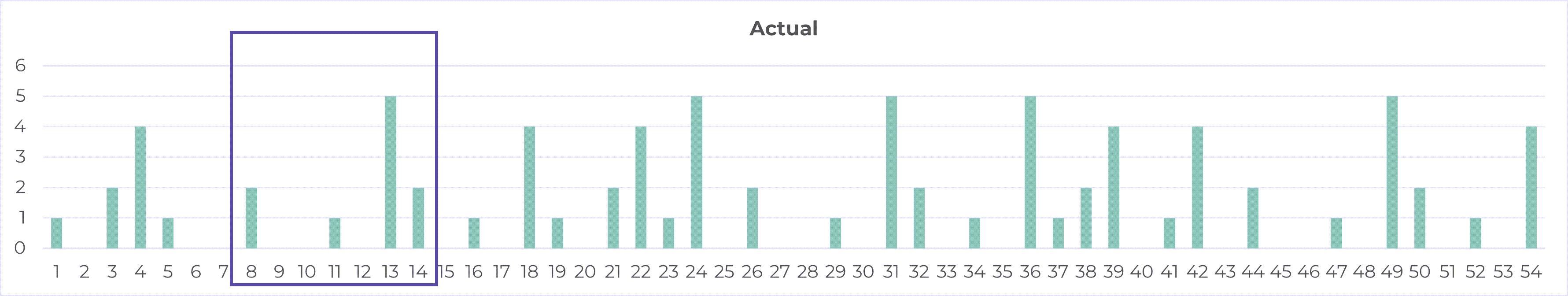
Figure 4
Click to enlarge
Figure 5
Click to enlarge
Figure 6

Click to enlarge
Figure 7

Click to enlarge
Figure 8

Click to enlarge
Figure 9
Click to enlarge
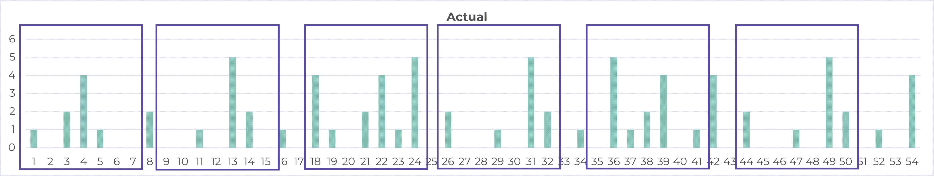
Figure 10
Click to enlarge
Figure 10 above is an attempt at summarizing the results of looking at the entire demand with a 7-day wide lens. Each purple box in the figure represents a 7-day window. Looking at the demand this way results in an average of 10.2 and a standard deviation of 2.91. (See Figure 11). This means that the standard deviation is less than a third of the mean, a significantly smaller amount compared to the calculation above. The average, when divided by 7 comes to 1.45, which is very close to the previously calculated daily average of 1.46. The standard deviation when divided by the square root of 7 comes to 1.10, which is much smaller than the previously calculated daily standard deviation of 1.70.
Figure 11
Click to enlarge
Until Next Time
Based on this, Jane put together a calculation to calculate the standard deviation of the demand over the lead time. The table below summarizes the calculations.
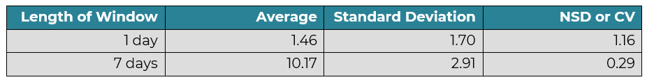
Click to enlarge
Kate suggested this was a good step forward but more needed to be done. Let us visit that in the next blog.

Read the next blog in the series here.