Introduction
Since the beginning of time, alternate but related views of production have existed: historically called “starts” and “outs”. The “starts” view dominates modern methods such as linear programming (LP). The “outs” view dominates older tools such as rough-cut capacity planning (RCCP) whose legacy is calculations on the back of an envelope. This blog provides a brief overview of the two views and how they are related.
Basics of Production Activity – “Starts” View
The core of any production or manufacturing activity is the decision to start a certain number of units of production with a certain manufacturing method (MM). A specific MM is called a manufacturing order (MO). The MM produces an item, product, or part, consumes component items, and consumes capacity of a manufacturing resource (MR). For simplicity, we will assume this MM does not consume a component item or that these items are trivial to obtain.
The amount a manufacturing resource (MR) consumes is based on the number of units started and the consumption rate or resource required (RR). If the RR is 2 and the number of “starts” is 100, then 200 units of the MR are consumed.
One additional part of the MM is “yield” – the fraction of the “starts” that can be used after the MM finishes. If yield is 100%, then when 100 units are started, 100 usable units are produced or manufactured – called “outs”. If the yield is 70%, then only 70 useful units are produced. Observe the amount of the MR consumed is a function of the number of units started, not the “outs”.
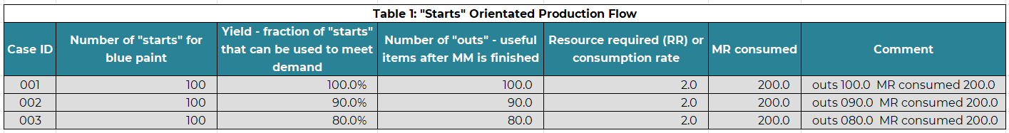
Table 1 has a “starts” orientation of the production flow. In the three cases, the number of “starts” is the same, 100, but the number “outs” is different since the yield declines. Observe that the units of the MR consumed is the same for each case. This orientation is typically for a linear programming formulation.
Business Focus Drives “Outs” View
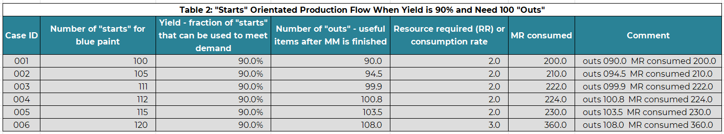
In Table 1, the decision focus is “starts”. If the firm “starts” 100 units, when the yield is 90%, the firm assumes it will get 90 units of usable “outs” to meet demand. This is “forward thinking”. However, the planner often begins with the question how to meet the demand for 100 units which drives the question how much capacity of the MR is needed to generate 100 “outs” – that is usable finished goods to meet the demand of 100. This “reverse thinking” is the orientation of an RCCP (rough cut capacity planning) model. One approach is to do a set of “what ifs” using the formula “outs” = “starts” x 90%. This is shown in Table 2. When 100 units are started (case 001), the “outs” is 90 – too little. When 120 units is started (case 006), the “outs” is 108 – too much. When “starts” is 111, the “outs” is 99.9 (essentially 100) – just right. Certainly, manually doing “what ifs” will take a long time. The question is can we do a little of algebra to calculate the capacity needed directly to get a certain number of “outs”? Yes.
Production Basics – “Outs” View
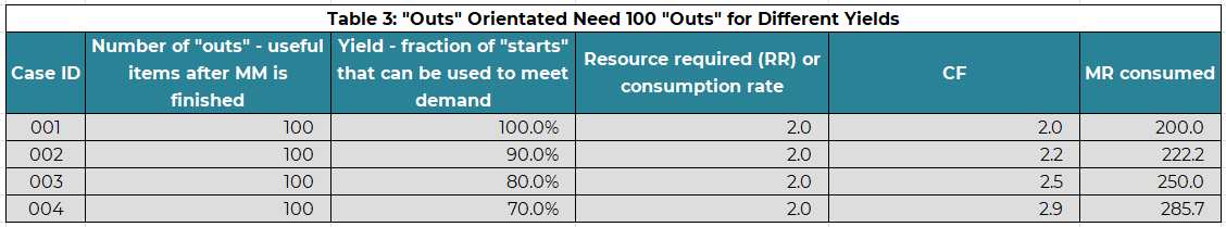
Table 3 has an “outs” or RCCP orientation to the MM. Observe the limitation of using just the CF is the loss of production information. It is impossible to tell if an increase or decrease in the amount of MR needed to generate a certain number of “outs” is a function of a change in yield or a change in the manufacturing process.
Summary
Complexity exists whether you ignore it or not. It is an inevitability the firm will need to know. The ongoing challenge is the firm will need to move to an LP or underperform.