Introduction
National Puzzle Day is January 29th. It is a day Arkieva celebrates because the ongoing challenge of smarter supply chain decisions involves supersized puzzles and games. Last year we wrote about Sudoku and optimization using binaries. This year we will focus on probabilistic forecasting using the board game Risk. This blog will show how Monte Carlo Simulation can be used to estimate the average number of “wins”, but critically the range of possible “wins” across some interval. In demand estimation terms, “average wins” is the point estimate for demand and “range of possible wins” is the likely variability in demand. You may find other puzzle blogs such as “Who’s Guilty?” and “Only the Shadow Knows” of interest.
Basics of Risk
The core of Risk and other board games such as Chancellorsville is moving your pieces from one area to another and then attacking your opponent. The wins and losses associated with an attack are determined by rolling die and comparing results between the attacker and defender.
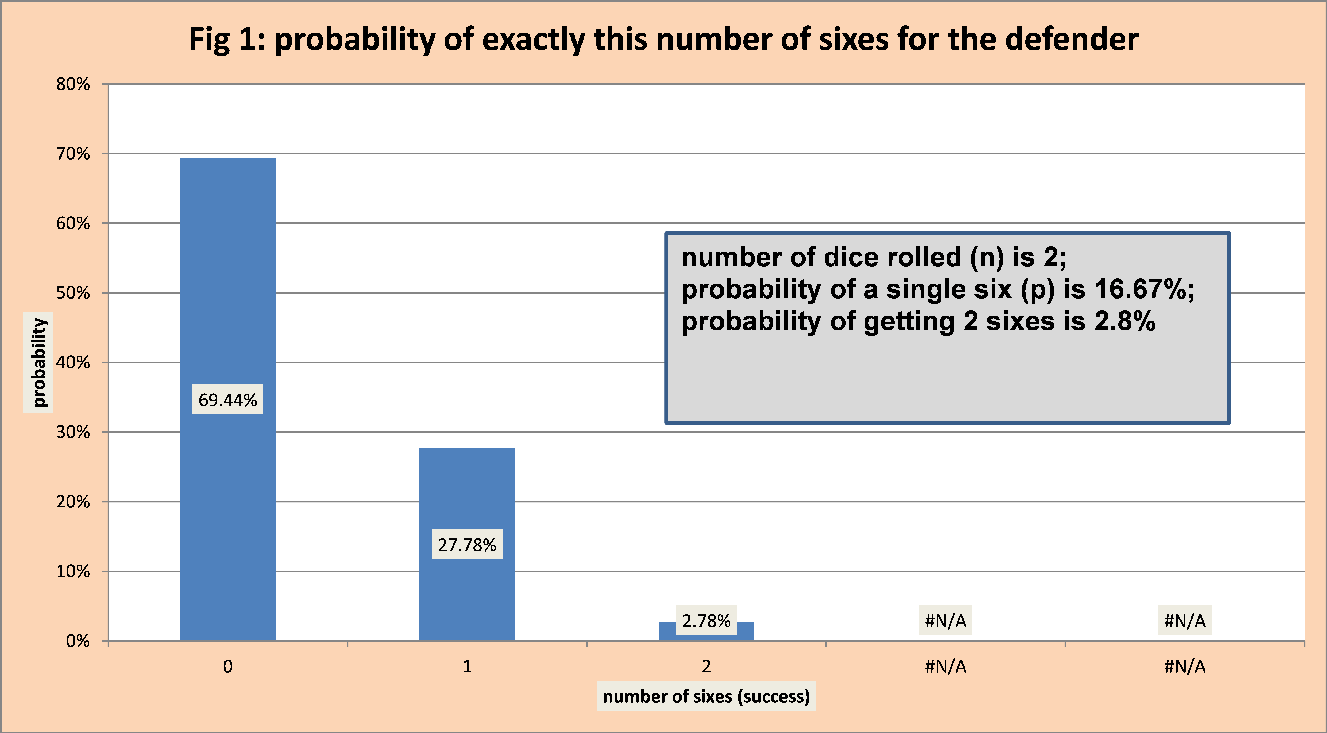
The defense rolls two die where the identity of each die is unimportant. The die are ordered high to low. For example, the defender might roll one 5 and one 4 – after ordering these rolls from high to low we get the pair (5,4). We can then use the binomial model to calculate the outcome of rolling exactly (0,6) , (1, 6), or (2, 6) . Figure 1 displays these probabilities. Notice the chance of getting two sixes is under 3%.
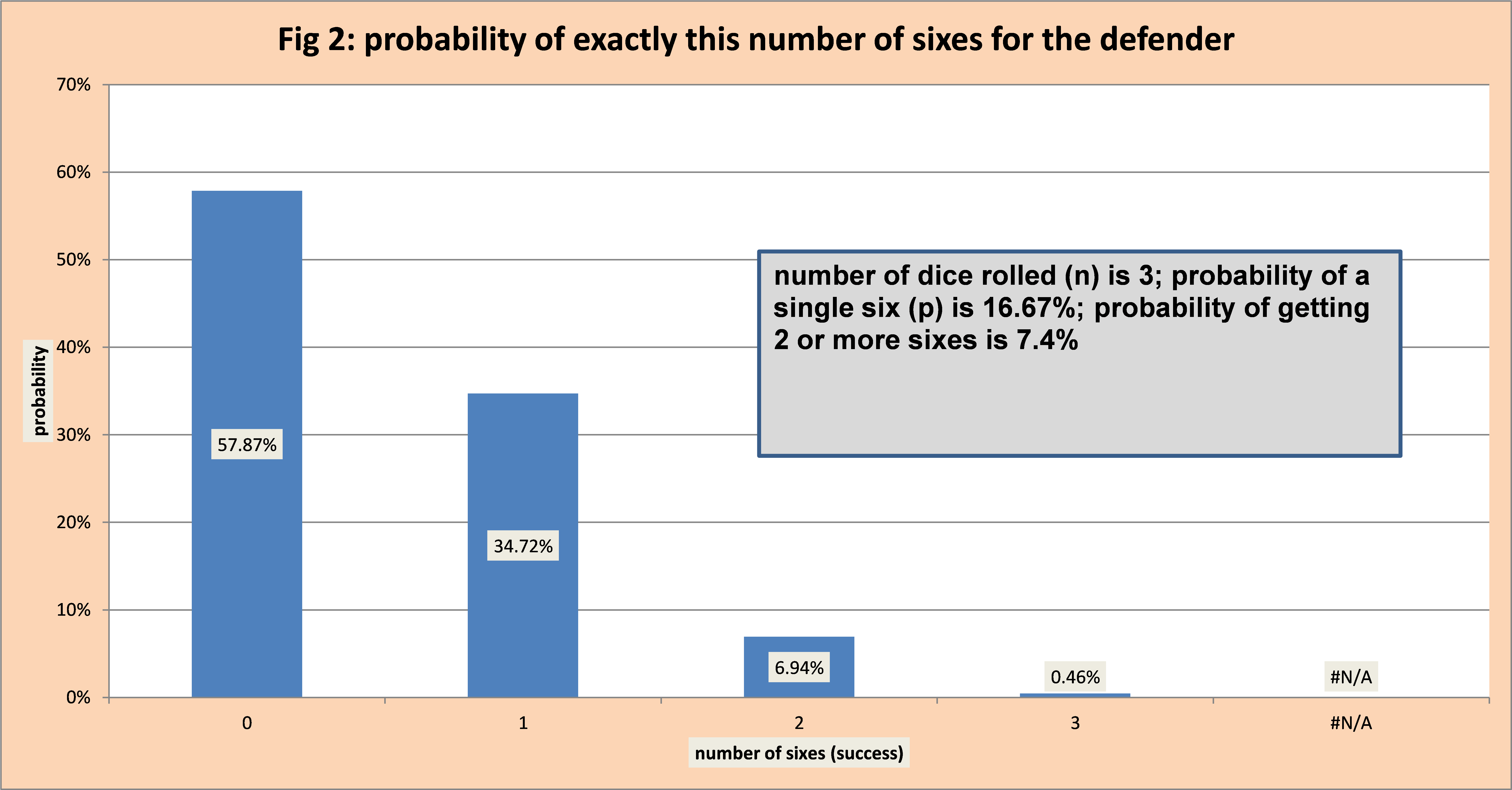
The attacker rolls three die which are ordered high to low, and the two highest values are selected for the competition. For example, the attacker might roll the values (4, 2, 6). When ordered high to low we have (6, 4, 2). The two largest values are selected giving us the pair (6,4). We will again use the binomial to calculate the probability of getting a six. Figure 2 displays these probabilities. The probability of getting 2 or more sixes (probability of 2 sixes plus the probability of 3 sixes) is 7.4%. We see the extra die is a large advantage.
How do we make the competition more competitive? If there is a tie, the defender wins. Let’s look at examples.
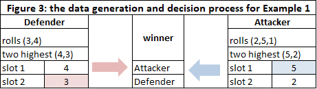
- Defender rolls (3,4) and attacker rolls (2, 5, 1). For the defender slot 1, the highest value is 4. Slot 2 is 3. The defender’s pair for competition is (4,3). For the attacker slot 1, the highest value is 5. Slot 2 is the next highest value which is 2. The attacker’s pair for competition is (5,2). We then compare the values in slot 1 for defender and attacker. Since 5 is greater than 4, the attacker wins, and the defender removes a unit from the board. We then compare the values in slot 2. Since 3 is greater than or equal to slot 2, the defender wins, and the attacker removes one unit. Loss summary is (1,1); one unit lost for attack and defense. Figure 3 illustrates this concept.
- Defender rolls (3,4) and attacker rolls (6, 3, 1). For the defender slot 1, the highest value is 4. Slot 2 is 3. The defender’s pair for competition is (4,3). For the attacker slot 1, the highest value is 6. Slot 2 is the next highest value which is 3. The attacker’s pair for competition is (6,3). We then compare the values in slot 1 for defender and attacker. Since 6 is greater than 4, the attacker wins. We then compare the values in slot 2. Since 3 is greater than or equal 3, the defender wins. Loss summary is (1,1).
- Defender rolls (5,5) and attacker rolls (6, 5, 5). For the defender slot 1, the highest value is 5. Slot 2 is 5. The defender’s pair for competition is (5,5). For the attacker slot 1, the highest value is 6. Slot 2 is the next highest value which is 5. The attacker’s pair for competition is (6,5). We then compare the values in slot 1 for defender and attacker. Since 6 is greater than 5, the attacker wins. We then compare the values in slot 2. Since 5 is greater than or equal 5, the defender wins.
- Defender rolls (4,5) and attacker rolls (6, 5, 5). For the defender slot 1, the highest value is 5. Slot 2 is 4. The defender’s pair for competition is (5,4). For the attacker slot 1 is the highest value which is 6. Slot 2 is the next highest value which is 5. The attacker’s pair for competition is (6,5). In this case, the attacker secures 2 wins for slot 1 and slot 2.
The critical question is who has the advantage the attacker (with 3 die) or the defender (wins ties)? This can be broken down into two questions:
- On average (that is with a very large number of attacks or competition) who has the most losses and by how much?
- What is the variation or probability distribution of comparative losses for a fixed number of competitions?
These are the exact two questions that arise in demand estimation.
Estimating the Comparative Loss and Variability using Monte Carlo Simulation
The most common and flexible method to acquire this information is Monte Carlo Simulation. Its use goes back to the 1950s and the advent of modern computers.
To do this simulation we write some quick code that does the following:
- Mimics the roll of the die for the defender and the attacker to get a roll set of each one.
- Some logic to select the two highest values for the attacker and defender to serve as the competition pair.
- Executes the “attack” which is the rules for comparing the competition pair.
- Keeps track of the loss for each combatant in a specific attack.
- Summarizes the results.
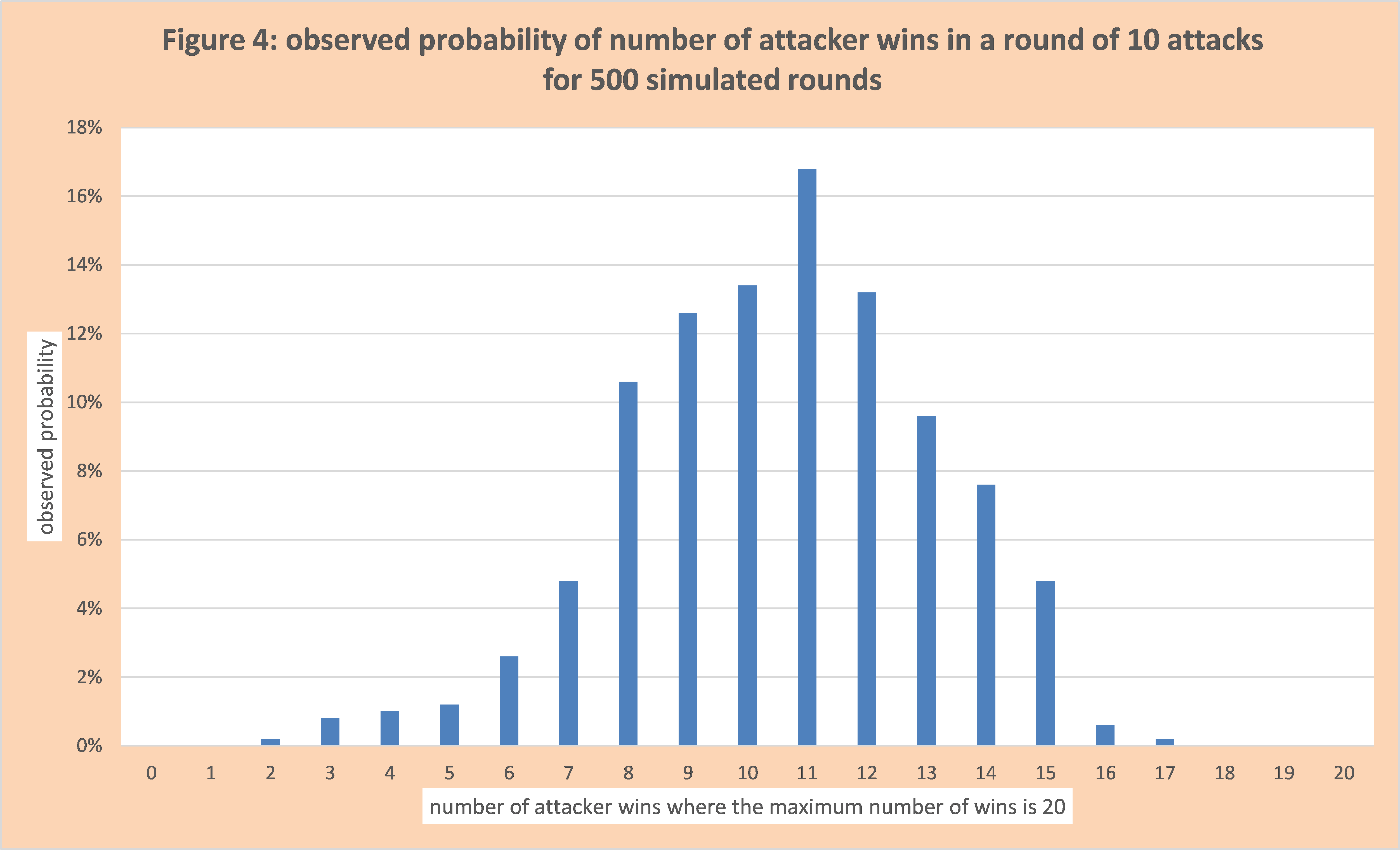
Using our code, we did a simulation to answer these questions. Each round of the simulation involved 10 attacks. That is 10 times we simulated rolling the die, identifying the competing pairs for defense and attacker, and determining wins. There was a maximum of 20 wins in a round (two pairs and 10 attacks). We simulated 500 rounds. In our first simulation set, the attacker on average had 10.82 wins per round. The defender had 9.18 wins per round. In the second simulation set, the attacker had 10.56 wins. To gain additional insight, we could increase the number of rounds from 500 to 1,000 to 10,000.
This information is a point estimate, that is on average with the current rules of who wins, the attacker has a slight advantage. The more interesting question is the variation between attack rounds, where the number of attacks per round is 10. This provides a picture of the risk. This information is displayed in Figure 4. For a sample of size 500 where each attack round consists of 10 attacks, the observed probability for the number of wins for the attacker is shown. Observe there is over a 30% chance the defender has more wins in each round than the attacker. This explains the wide-open nature of Risk when it is played.
Conclusion
Although games and puzzles are often viewed as “less than good use of time”, they often inspire an understanding and solutions for “serious” challenges in managing demand supply networks. In this blog, the simulation model provided insight into the wide-open nature of Risk where the complexity of the rules of who wins and rules are not intuitive. This example makes clear of the importance of models and the power of simulation to provide insight into complexity to support critical decisions.