Only the Shadow Knows – Identifying the Unobvious with Supply Chain Modeling

The importance of the right toolkit to understand the non-intuitive aspects of supply chain management

While reading a wonderful article titled “Linear Thinking in a Non-Linear World – the obvious choice is often wrong” in the May-June 2017 issue of Harvard Business Review, I was immediately transferred back to the early 1980’s and theme of the IBM Advanced Industrial Engineering department – “only the model knows.” This was a take-off from a famous radio show in the 1930s which started – “Who knows what evil lurks in the hearts of men? The Shadow knows. Evil, being replaced with three non-intuitive aspects found in planning:

Non-Linearity
Complex systems are generated by the relationships among simple components
Probability

“Computational Models” being the critical toolkit to help the planning and management team get a clear picture of the supply chain – the equivalent of saws, nails, and a hammer for a carpenter.

Understanding the Non-Intuitive Aspects of Supply Chain Management with Supply Chain Modeling

To understand item 2, we will start with the initial question posed in the HBR article you manage a fleet of vehicles that have 5 SUVS getting 10 MPG and five sedans getting 20 MPG; each vehicle travels 2,000 miles per year. You have enough capital to replace all of the SUVs or all of the sedans with more-fuel-efficient vehicles. The initial question is which of the following upgrades is better?

A. Replacing the 10 MPG vehicles with 20 MPG vehicles

B. Replacing the 20 MPG vehicles with 50 MPG vehicles

Often the initial observation is B is the better choice since it has the largest increase in MPG. Let’s stop and think of the parts and their relationship.

Identify the business goal and its metric – reduce the number of gallons of gasoline purchased. The following model (table) answers this question

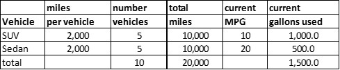
The SUV fleet requires 1,000 gallons of gasoline, and the sedans’ require 500.

What are the components – miles per vehicle, number of vehicles, and MPG?
What is the current component we need to make a decision about? – MPG
What is the impact of a change in MPG? The following table model helps us make this assessment

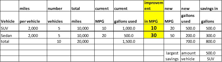
The decision variable is identified in yellow – “improvement.” The new MPG is the old MPG plus the improvement. We see a 10 MPG improvement for the SUV generates far more saving than the 30 MPG for the sedans. The model (tool) captures the relationships among simple components (miles driven, MPG, and savings) to make the correct business assessment – improve MPG for the SUV. It also provides some key insights that our mind does not immediately conjure up. The maximum gallon savings for Sedans is one-half of that for the SUV.

Quickly we can generate other scenarios that could reduce gallons used and evaluate them with the model. For example, reduce the number of SUVs to 3, increase their miles per car to 2500, and the MPG increases by 10; purchase two additional sedans where the average number of miles is now 1800, and invest in 10 MPG improvement in sedans.

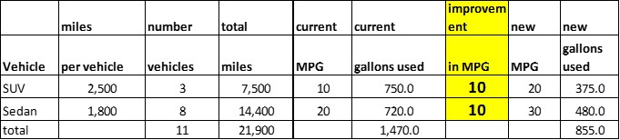
This reduces the total gallons used from 1,500 to 855. The first option reduces total gallons to 700. However, the second might be cheaper!

What if we have lots of scenarios to evaluate or we have some broad outlines of “stuff we can change” subject to certain limits. This leads us to the “advanced” toolkit – called optimization. At Arkieva, we help our customers build optimization models that can analyze different scenarios and help them determine the best outcomes in relatively short amount of time.

What About Probability?

Now that we’ve addressed the concept of generating complex systems by looking at the relationship among simple components; let’s turn our attention to probability.

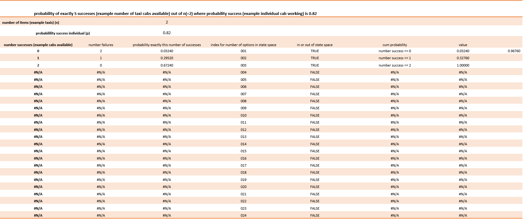
A real example – simplified. The manufacturing manager has to purchase machines to support production and has two options.

The manager can purchase one machine with a reliability of 95%, and as long as this machine is working, the factory can meet its critical demand.
The manager can purchase two machines, each of which has the reliability of 82% and as long as at least one machine is working, the factory can meet its critical demand.

The metric is what percentage of time the factory will be able to meet its critical demand. Which is the best option? With an initial inspection, one might select option A.

For option A, the answer is obvious – 95%.

What about option B? There are three ways critical demand can be met

Machine 1 is working; Machine 2 is down
Machine 1 is down; Machine 2 is working
Machine 1 is working; Machine 2 is working

The binomial model comes to rescue and tells us option B can meet critical demand 96.7% of the time.

The key takeaway is, like all tools, computational models can be very helpful in the right circumstances, and it can be almost impossible do some tasks without the right tools.