In Part 1 of this blog, we closed with the following question: “OK, intermittent demand creates a challenge, but I still need a demand estimate, what do I do!” Below we will provide an answer, but with a different orientation that begins with the question: “what is the purpose of the demand estimate?” The demand estimate has three primary purposes:
- An estimate of the financial position of the organization.
- An estimate to drive the acquisition of product to place in inventory (inventory replenishment) to meet demand, where acquisition may be purchase or production.
- An assessment of resources required, where a resource may range from storage space to labor.
We will focus on question 2- inventory replenishment.
Read More: How to Measure Forecast Errors in Intermittent Demand Forecasting
We will continue to use the intermittent demand example from the first blog. The probability of getting a nonzero demand value on any given day is 20%, the probability of zero demand is 80% (=100%-20%). If there is demand, the possible values are 1, 2, or 3 (with equal probability). The average demand on non-zero days is 2 (=(1+2+3)/3=6/3). The average demand per day is 0.4 (=0x(0.8) + 2x(0.2)= 0 + 0.4).
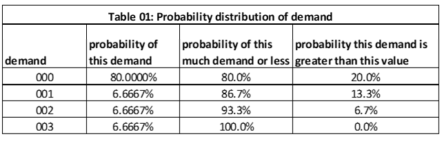
Table 01 has an alternative and very helpful, way to capture the probability of demand.
Row 4 (demand of 001) tells us the probability of demand is equal to 1 on any given day is 6.6667% (column 2), the probability that demand is 1 or less is 86.7% (column 3). The probability demand is greater than 1 this day is 13.3% (column 4).
Our product is cherry butter pecan (CBP) 1/2 gallons of ice cream, where the lead time to replenish inventory is overnight. An inventory replenishment request is made at the end of the day and the inventory arrives at the start of the next day. If I reorder 10 units at the end of day 1, then the 10 units will arrive at the start of day 2 and available to sell. The key questions are:
- How much to hold in inventory?
- How often to reorder?
For simplicity we will assume the cost to reorder is zero, the cost to hold inventory is $1 per day, the revenue for each sale is $3, the probability the new order arrives on time is 100%, the shelf life of a unit of CHP is 100 days, and the limit on storage space is 100 units. If a customer comes to the store to purchase CBP and there is no CBP (stockout), the order (sale) is lost forever. Since reorder cost is 0 and the reorder lead time is overnight, the critical question is how much inventory to hold at the start of each day, which is a question of managing the risk of a lost sale versus holding cost.
How much to hold in inventory at the start of the day? We know the minimum demand each day is 0 and the maximum demand for a day is 3. The options are 0, 1, 2, and 3. If my target inventory level for CBP is 0, then I am essentially not selling this product – so this option is eliminated.
What about holding 1 unit? What is the probability I will meet all the demand for this day? If demand is 0 or 1, then all demand is met? If demand is 2 or 3, then sales are lost. What is the probability I will have inventory left at the end of the day? If demand is 0, I will have 1 unit left. If demand is 1, 2, or 3, I will have no inventory left.
What is the revenue and costs for having one unit in inventory and demand is 0
- Revenue from sales is $0 = (0 x $3)
- Holding cost is $1 = (1 x $1)
- Net position is $-1 =$0 – $1
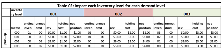
Table 02 summarizes the business outcome for each demand and starting inventory combination for five key metrics: ending inventory, unmet demand, revenue, holding cost, and net position.
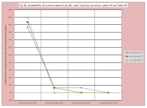
We still need to make a decision on how much inventory to hold! Assume the two key metrics are unmet demand (client satisfaction) and ending inventory (business target of ice cream freshness). Then we can create a risk profile for each inventory option for each key metric. Table 03 has the probability of an unmet demand level for each starting inventory level. Table 04 has the probability of each ending inventory level for each possible starting inventory decision. Figures 01 displays the information in Table 03 graphically making clear the non-linear nature of the relationship between starting inventory and unmet demand.
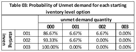
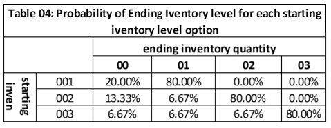
The decision-maker simply selects a starting inventory level based on their risk preference for unmet demand and ending inventory level. The tables have all the options. The reader will clearly see there is no “free lunch”. More starting inventory would likely mean higher ending inventory, but a lower chance of unmet demand. For example, a starting inventory level of 1 has about a 13.4% chance of some unmet demand, but no chance of ending levels greater than 1. If the decision-maker selects a starting inventory level of 2, the chance of unmet demand drops to 6.67%, but now has an 80% chance of an ending inventory level greater than 1. In practice (for example, see LMI paper), a front end is built to support the business decisions and display the risks and costs.
Observe, we have generated all the core components (options, consequences, and risk or probability) to make a key inventory replenishment decision without ever generating a detailed demand forecast.
The decision-maker identified freshness as a business objective. A question the decision-maker might ask is if I have one new unit of CBP in inventory, what is the chance this unit will go unsold for 3 days. We know the chances it will go unsold for one day is 80% since the probability of zero demand on any given day is 80%. This risk can be calculated using standard methods. The probability of zero demand for three successive days is 51.2%. If there are two new units of CBP in inventory, what is the chance at least one will go unsold for 3 days, this is 64%. Again, a critical risk decision can be assessed without ever generating a daily demand estimate.
Summary
Demand with lots of zeroes requires special attention and expertise. There are two major types: structural and intermittent. Intermittent implies the pattern of zeroes is random and requires special attention. The information presented above attempts to make clear the key to success is changing your orientation from detailed estimates to incorporating risk trade-offs which is in alignment with the origins of forecasting (p. 95 Against the Gods, the Remarkable Story of Risk by Peter Bernstein). Of course, business trade-offs are more complicated than this simple example. Organizations that have adopted this approach have seen significant benefits.
Effective Inventory Control for Items with Highly Variable Demand
Enjoyed this post? Subscribe or follow Arkieva on Linkedin, Twitter, and Facebook for blog updates.