How to Measure Forecast Errors in Intermittent Demand Forecasting

Intermittent Demand Forecasting Accuracy Metrics: Key Takeaways

Understand if the product has structural zeros or intermittent zeros
Structural zeros have a noticeable data pattern whereas intermittent zeros occur randomly
Do not use standard metrics for measuring forecast accuracy
Track the probability of demand occurring across time in place of traditional forecast accuracy metrics

It has been estimated as many as 50% of products and services have demand patterns with “lots of zeroes”, which creates special challenges for demand estimation and the failure to handle “lots of zeroes” correctly can cripple the effectiveness of an operational process from hospital pharmacies to forecasting intermittent demand for car spare parts.

The purpose of this blog is to provide basic information on intermittent demand (defined below) making the following guidelines easier to understand:

Standard metrics for forecast accuracy are not only wrong – they will get you into a lot of trouble and mess up your business
The key metric is business impact and what is needed is a risk profile – the probability of demand occurring across time, or possible lead time

It is very helpful to divide products with “lots of zeroes” into two groups

Structural zeroes – the zeroes have a pattern that relates to the structure of the supply chain or data collection methods.
Intermittent / Sparse / Lumpy – demand has lots of zeros spread randomly across time

Structural Zeroes

The examples in this blog will assume four years of demand history where the time bucket is months. This is 48 total observations. Tables 1, 2, and 3 provide examples of structural zeros.

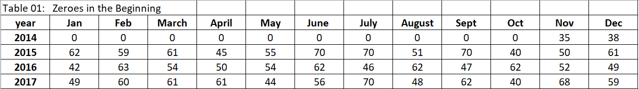
Table 1: The zeroes are at the start of the history – indicating the product was not active at this time or the demand data was not collected. Often a “zero”, as opposed to null, is used as filler.

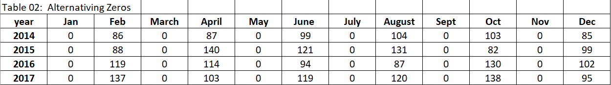
Table 2: Every other cell is zero, this often occurs if the demand collection system only grabs demand every other month.

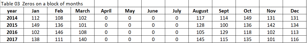
Table 3: Has zeroes in a block of months (April – August). This would indicate a structural item that drives demand to ZERO during this time period – for example, if the demand for flu shots.

Intermittent Zeroes

Intermittent (other terms used are sparse and lumpy) refers to demand patterns where there are many zeroes (typically at least 50%), the dispersion or location of the zeroes does not show a particular pattern (random), and the non-zero values have a range of values without an apparent pattern.

When a statistician uses the term “random”, it means assuming random is the best we can do given the information available and any discernable pattern that can be found in the current data. It does not mean there is no cause for a zero or non-zero, simply this is the best we can do right now and it is optimal to deploy methods that provide insight with this assumption.

How do we know if the assumption of random is reasonable for a given data set? The non-parametric statistical method called a run test is a powerful method (see “Nonparametric Statistical Inference” by Gibbons and Chakraborti). A run would be defined as a succession of 0s or non- zeroes data set. For example, in the data set 0 0 0 0 0 1 1 1 1 1, there are 10 members and two runs. In the data set 0 1 0 1 0 1 0 1 0 1 there are 10 members and 10 runs. In the data set 1 1 1 0 0 0 1 0 0 1 there are 10 members and 4 runs. When the number of runs is too small or too large then we conclude the data, the set is not random.

For our example, we will assume the probability of getting a nonzero demand value is 20% and if there is demand, the possible values are 1, 2, or 3 (with equal probability, an average of 2). If the total observations are 48, on average the number of nonzero cells will be 9.6 (=0.2*48) and the average demand value will be 0.4 = ((0.2 * 48 * 2)/48) = (0.2 * 2).

Example Intermittent Demand Forecasting Techniques for Determining ‘Best Estimates’

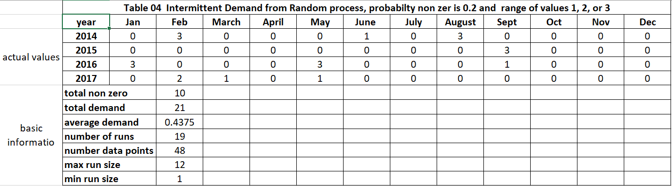
Table 4 has a randomly generated set of intermittent demands. How might we best estimate demand for each cell (year and month)?

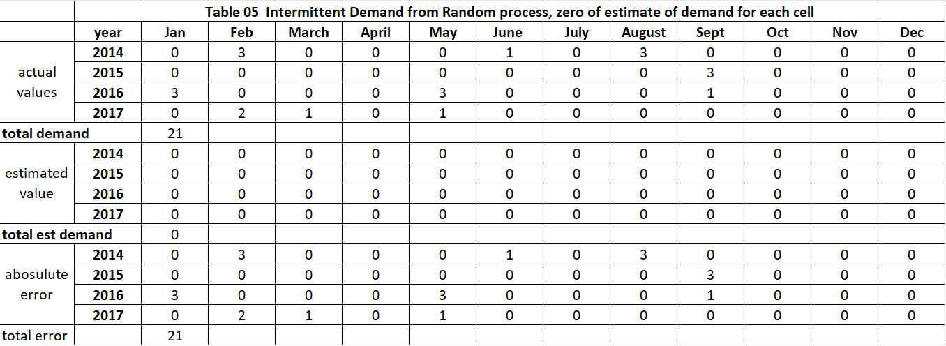
Table 5 summarizes how “well” using zero as an estimate for each cell works. The actual demands are in rows 3 to 6, the estimated demand of zero is rows 8 to 11, and the error metric is in rows 13 to 16. The metric used is total absolute error. For each cell, we calculate the absolute value of the actual value minus the estimated value, then sum across each year and each month. We see “zero” has a low forecast error – a total of 21.

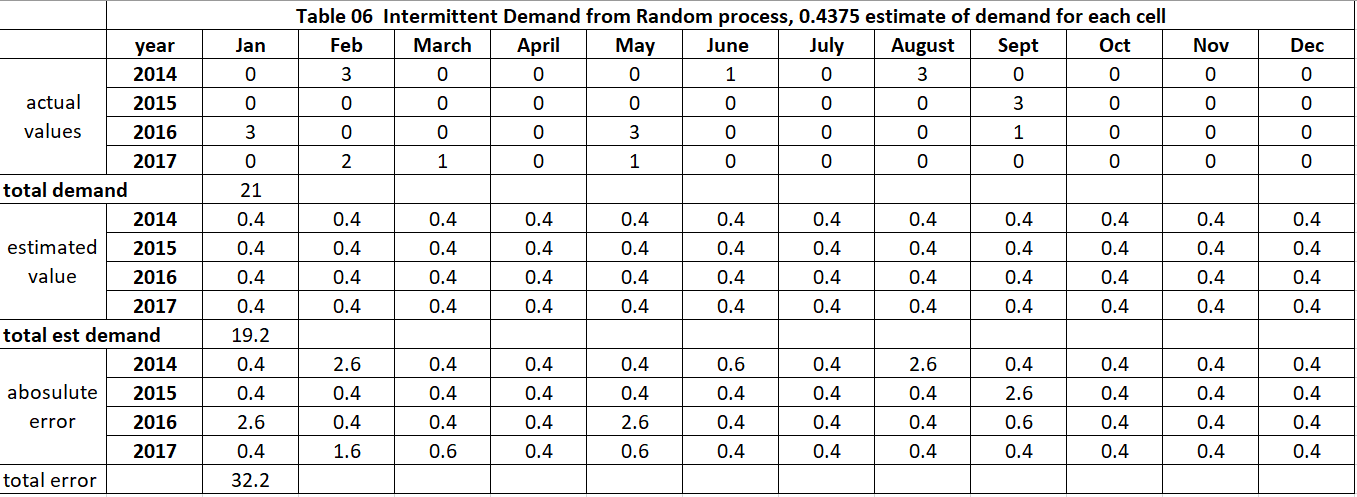
Table 6 summarizes how well using the average value (0.4) does. Its error metric value is 32.2.

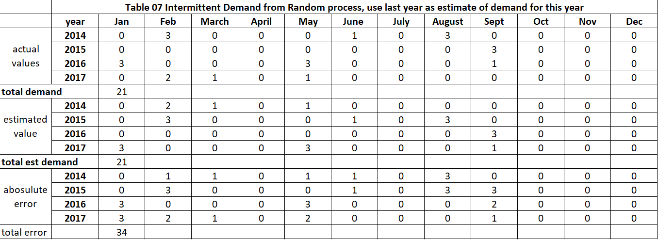
Table 7 summarizes if how well using last year to estimate this year works, its metric is 34.

Observe the intermittent demand estimate of “zero” works much better than the two alternative methods based on a standard forecast error metric. However, relying on the standard metric to identify the right forecast method will be disastrous to the firm. To understand this, compare the total actual demand versus the total estimated demand. The “zero” method will instruct the firm to produce or acquire zero of this product. Note the other two methods do much better at estimating the aggregate demand.

What we need is a metric this is reasonably easy to understand but captures the probability of a certain level of demand by a specified point in time. For this, we will use cumulative demand.

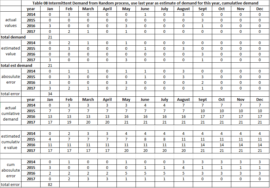
Table 8 demonstrates the cumulative demand. Rows 19 to 22 have the cumulative actual demand to date. The value of 7 in the cell (2014, August) means the total demand since (2014, Jan) is 7 – 3 from Feb, 1 from June, 3 from August. Rows 24 to 27 have cumulative estimated demand. The value of 4 in the cell (2014, August) means the total estimated demand since (2014, Jan) is 4 – 2 from Feb, 1 from March, 1 from May.

The cumulative error metric can be tweaked based on business need. Is the estimate needed for inventory replenishment or to generate production starts? The metrics should be tuned based on business need. For example, for a new product, there may be a new machine in the factory – called an OAK (one of a kind), the estimate should be tuned to provide insight into expected utilization of the OAK tool.

The last method (table 7) used to generate an estimate of demand is to use the last year. A better and more robust method is resampling or bootstrapping – a topic for another blog.

Summary
Demand with lots of zeroes requires special attention and expertise. There are two major types: structural and intermittent. Intermittent demand implies the pattern of zeroes is random. Traditional metrics of forecast accuracy can result in destructive behaviors. The key is to treat the estimation process as a risk trade-off. Firms that can do this well, will see a large improvement in performance.

Enjoyed this post? Subscribe or follow Arkieva on Linkedin, Twitter, and Facebook for blog updates.