In my last post, I talked about the relationship between the mean absolute deviation (MAD) and standard deviation (STDEV) for a normal distribution. Apparently, many people had never seen the math behind it, and I got questions about the same relationship for the case where the demand was not normally distributed. In this post, I am going to derive the same for a uniform distribution.
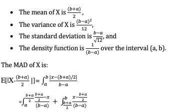
Say X is a uniformly distributed random variable between limits a and b. Then:

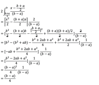
By symmetry, the two integrals are equal, so we can just evaluate:

Read More: How to Report Forecast Accuracy to Management
MAD = (b – a)/4
The ratio of MAD to standard deviation is:

Thus, MAD ≈ 0.866 (ST DEV)
Or ST DEV ≈ 1.155 (MAD)
By referencing the previous blog, we can see that the relationship between MAD and Standard Deviation for a normal distribution is:
ST DEV ≈ .1.25 (MAD)
This goes to show that the underlying distribution matters and one should not blindly use one value to estimate the relationship between the two.
Read More: Seasonal Model Forecasting with Seasonal Methods
Enjoyed this post? Subscribe or follow Arkieva on Linkedin, Twitter, and Facebook for blog updates.

Dr. Tenga has more than 43 years of experience in all aspects of analytics especially in complex optimizations involving matching assets with demand, simulation, and forecasting, especially the application of optimization methods for next-generation demand estimation. He and Dr. Fox were the first two Arkieva hires when the firm was started in 1993. He has done optimization models for most Arkieva clients, including but not limited to, INEOS, Momentive, Hexion, Anadigics, Grande Cheese, Sunsweet, Dell, Philips, Advanced Drainage Systems, and SPI. He is the gold standard for Industrial Strength Optimization (ISO) expertise easily handling such complexities as decomposing optimization of the entire challenge into a set of tightly coupled optimization models, models with restrictive requirements (for example can only make 3 types of cookies in a given time bucket for the first 6 weeks) early in the time horizon, full date effectivity, variable size time buckets, frozen zones, filling tanks, capturing the cost and setup time for production changeovers, borrowing time between time buckets, shelf life, target cheese ages, and many more. Easy being defined as successful and the user can understand the results. Before joining Arkieva Dr. Tenga was a senior analytics professional at Dupont. Bob received his Ph.D. from Cornell University and B.S in mathematics from MIT.


