
In the previous What-if Wednesday posts, we experimented with the three parameters of the Holt-Winters Multiplicative method, namely; alpha, beta, and gamma. This time we are going to run similar tests by adjusting damping factor for the Winters Multiplicative method.
As discussed in the Winters Additive method blog on damping factors, a damping factor is an additional parameter that forecasting tools use to damp the forecast. This usually affects the trend of the forecast. Usually, we do not expect sales to grow year over year with the same increasing (or decreasing) trend. When this happens, we need to damp the forecast that was created using the historical trend. Its value can be set to any number between 0 and 1. The idea here is that when the damping factor is set to 0.9, the trend in the forecast will be reduced to 90% for each future period.
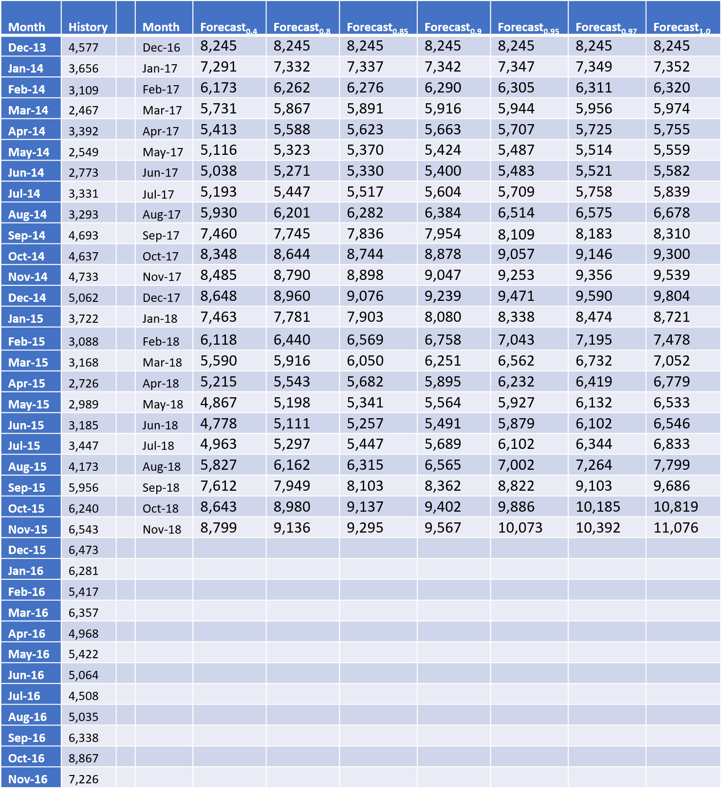
To experiment, we used a seasonal dataset that has a slight upward trend and applied the Holt-Winters Multiplicative forecasting method with varying damping factors. For our simulation, we have set the alpha, beta and gamma values to 0.05 and have varied the damping factor from 0.05 to 1 to understand its effect on the forecast. We could only see an appreciable change in the forecast when the factor was 0.4 and above. So, the charts below show the forecast based on different damping factors as we go from 0.4 to 1. The actual forecast numbers are at the end of the post.
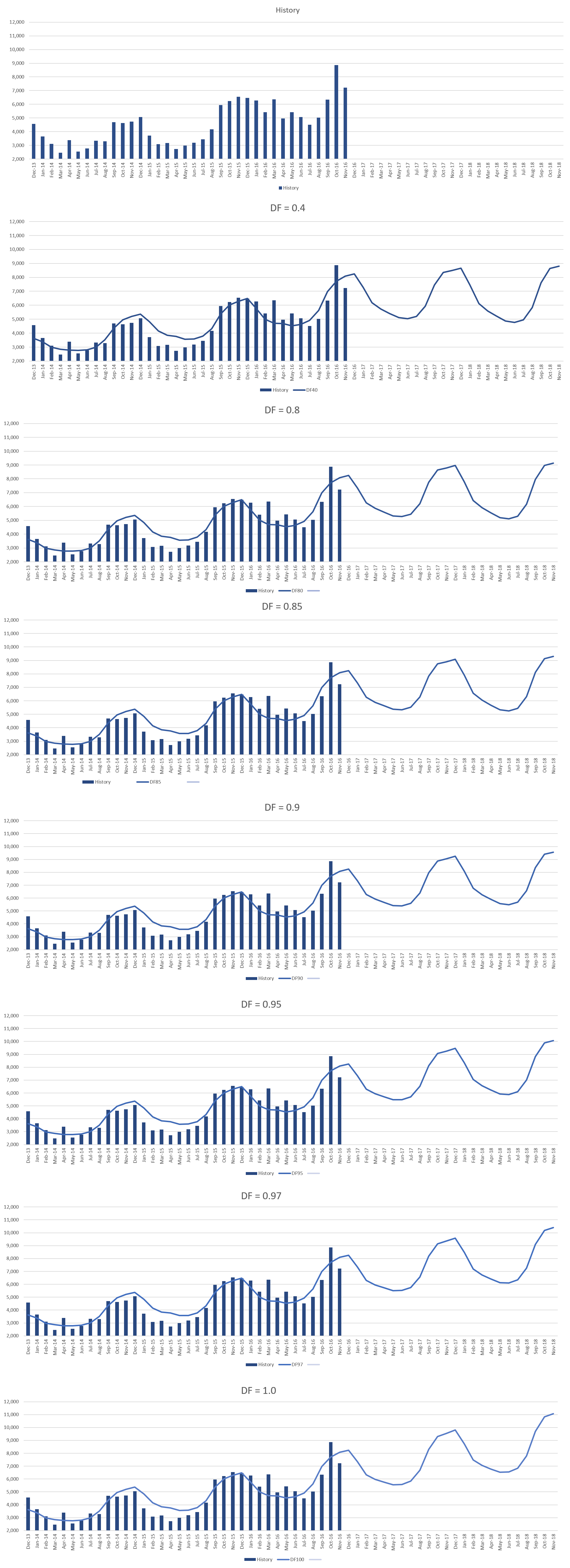
The overall behavior of the forecast with the changing damping factor is similar to what we saw with Winter’s Additive method in the previous blog. With damping factor set to 0.4, we see the trend doesn’t pick up much from its historical trend, meaning essentially no increase in the next two years. And, as the factor is increased from 0.8 to 0.85 to 0.9 we see an uplift in the trend which is more in line with the history. In the last chart, with damping factor set to 1, the forecast continues with the same trend with no damping at all. Compared to the Winter’s additive method the trend change with this method is sharper since the variations are proportional to the level.
Ideally, we would not want to have a very high damping factor unless we are highly certain that the sales are going to continue to grow at this pace even far ahead into the future. We also do not want to keep it so low that the valuable trend information is lost. Typically, we keep it around 0.8 to 0.9 range so that it captures the trend along with a slight damping to be on the conservative side while forecasting.
Enjoyed this post? Subscribe or follow Arkieva on Linkedin, Twitter, and Facebook for blog updates.