Key Point: Coefficient of Variation is not a perfect measure of forecastability. However, if used properly, it can add value to a business’s forecasting process.
In the world of forecasting, one of the key questions to consider is the forecastability of a particular set of data. For example, a salesman might consistently be better at forecasting compared to his or her colleague. Is this because the data assigned to them is more forecastable, or is the salesman in question more skilled at forecasting?
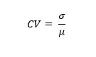
One of the ways demand planners have tried to answer this question is through the use of a calculation called Coefficient of Variation (CV). Some people call it standardized or normalized standard deviation (StdDev). In layman’s terms, Coefficient of Variation is a measure of how closely grouped a particular data set is. The formula for CV is:
CV = StdDev (σ) / Mean (µ).
In this blog post, I will shed some light on this particular measure and how to interpret it.
A key value of the CV is it adjusts for the differences in magnitude – it measures spread relative to magnitude.
- Case 1: Mean = 50; StdDev = 01, CV = 01/50 = 0.02
- Case 2: Mean = 5000; StdDev = 50, CV =50/5000 = 0.01
Based just on StdDev, case 2 appears to have a bigger spread, but looking at CV, we recognize that it is less of a spread compared to its magnitude. Lower CVs always represent narrower spread.
NOTE: It is true that CV does not apply to all types of data. For example:
- Sporadic or intermittent data cannot be analyzed for forecastability using this particular measure.
- Seasonal data might have a high CV but could be very forecastable.
- This measure completely ignores the sequence of observations. A perfectly trending set of numbers might get tagged as unforecastable because they have a high CV.
While not perfect, this measure remains very popular among practitioners, perhaps because it is very simple to calculate. In this post, I am limiting myself to explaining how CV should be interpreted and not focusing too much on its weaknesses.
Now let us look at a few examples: The table below shows three rows of data.
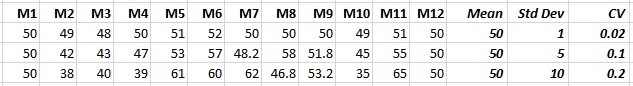
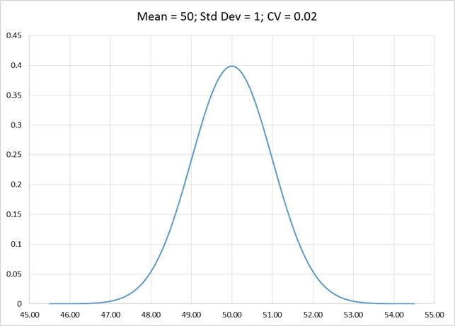
The first chart below shows the data corresponding to the first row (Mean = 50, StdDev = 1, CV = 0.02). As you can see, the distribution is quite narrow. This means that the job of the forecaster is quite easy. If it were me, I would make the forecast 50 in all future months.
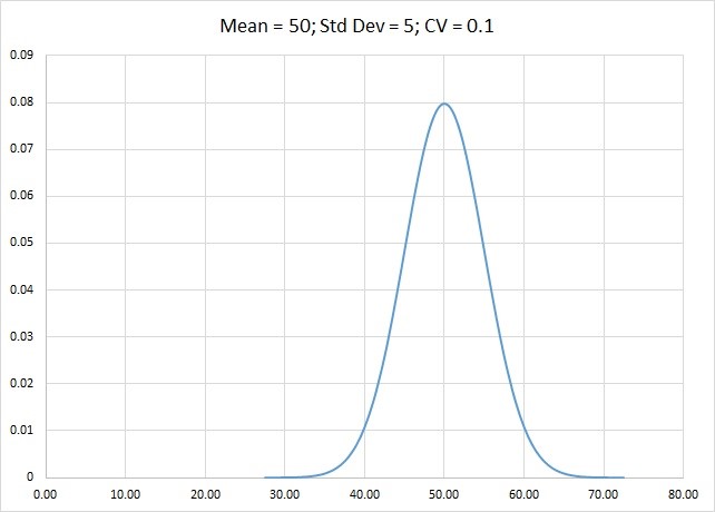
The next chart represents the data in the second row (Mean = 50, StdDev = 5, CV = 0.1). When compared to the example above, the forecasting is a little bit more difficult, because of the wider spread.
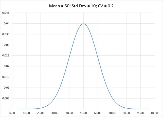
The next chart represents the data in the third row (Mean = 50, StdDev = 10, CV = 0.2). As you can see, the spread is wider. And compared to the two distributions above, the data is more difficult to forecast, because of the even wider spread.
So, if we put different CVs on the same graph, a picture emerges that is worth a second look. I have plotted a CV of 0.15, 0.3, 0.5, 0.7, 1, 1.5 and 2 on a mean of 10,000. Results are in the chart below.
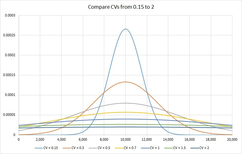
As you can see in the picture above, a CV of 0.15 has most of the data near its mean and therefore highly forecastable. On, the other extreme, a CV of 2 is so flat, it only remotely resembles our standard view of the bell curve. Forecasting will be very difficult on such a data set.
Based on the graph above, one can say that lower CV values would mean greater predictability on account of a tighter distribution. In my work with Arkieva clients I typically do the following:
- Using upfront analysis, divide the data into two sets – one where CV is relevant, and other where it is not (see the note above). Then, in the first data set, I do the CV calculations.
- I like to use a cut off of 0.3 as a measure of high forecastability.
- I consider anything above a CV of 0.7 as highly variable and not really forecastable.
- The cutoff values (0.3 and 0.7) are somewhat arbitrary and you might want to use slightly different values.
Do you use CV in your business? If so, I am interested in hearing from you.
Like this blog? Follow us on LinkedIn or Twitter and we will send you notifications on all future blogs.