Summary

In many areas of supply chain management, analytic methods generate estimates with “pesky decimals”; for example, demand estimates and production planning. The traditional method to eliminate pesky decimals is rounding. However, this also results in the loss of critical information the cumulative sum, which can often either understate or overstate workload on the firm. The rolling rounding method caps this information loss at 1. This blog demonstrates the importance of this method and how to calculate these improved integer estimates.

Introduction

While spending time with the “munchkins” (grandchildren) it is clear why the positive integers (perhaps with zero) are referred to as the natural numbers; counting is intuitive. This same comfort occurs in supply chain management. If the time series forecasting method predicts daily demand of 3.1, 4.2, and 2.3 – our preference becomes to rid ourselves of those pesky decimals.  If the product plan says the daily production should be 2.9, 3.1, and 1.7, we have the same feeling. The question is how best to eliminate the decimals, where best is defined as minimizing the amount of lost information.

[cta id=’4922′]

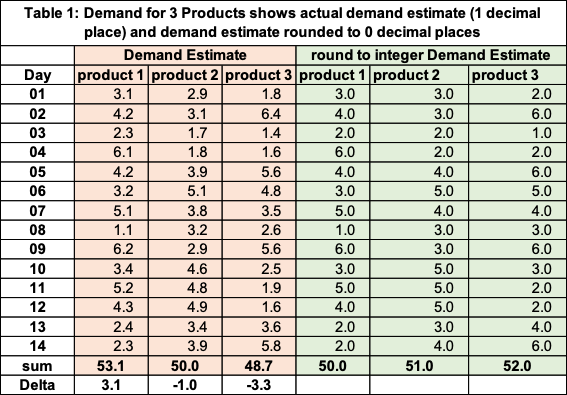
The traditional method is to round each individual value to an integer and assume the “rounding errors” will balance out. However, this is not always true. Table 1 has 14 days of demand estimates for three products (product 1, 2, and 3). The actual demand estimates are in columns two, three, and four. The sum of demands for each product (53.1, 50.0, and 48.7) are provided in the next to last row. The rounded demands are in columns five to seven and their total is in the next to last row (50, 51, 52). The last row shows the detail between the sum of the actual estimates and the sum of the rounded estimates. There is a sizeable difference for product 1 (3.1) and product 3 (-3.3).

What we need is a “rounding” method that bounds the difference in the cumulative sums to 1 and ensures the cumulative sum of the rounded values is greater than the cumulative sum of the actual values. This is called “rolling rounding”. This blog provides an algorithm for rolling rounding. It is part of the series on Data Science Tools of the Trade.

Machine Learning and Data Science Tools of the Trade: First-Order Difference

Tools of the Trade: How to Compare / Combine Diverse Time Series – “Normalizing”

Data Science Tools of the Trade: Monte Carlo Computer Simulation

Basics of Rolling Rounding

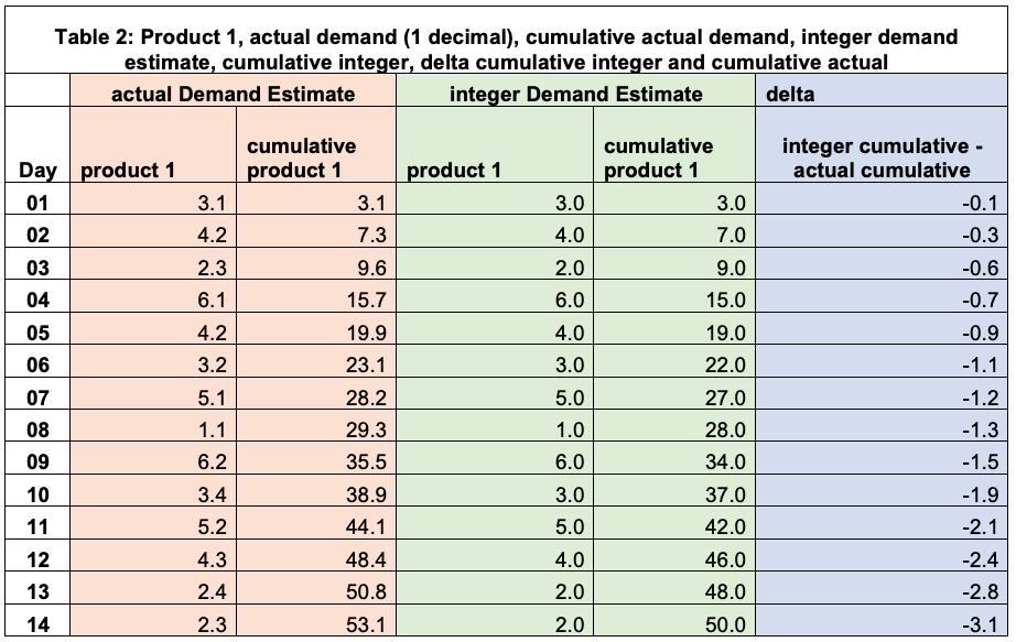
We will start with an example of cumulative sum.  Table 2 has the demand estimate for product 1 and the cumulative sum for actual and integer estimate. Column 3 is the cumulative actual. Day 1 is the demand estimate for day 1.  Day 2 is the cumulative sum from Day 1 (3.1) plus demand estimate for day 2 (4.2) which is 7.3.  Day 3 is 7.3 + 2.3 = 9.6 Column 4 is the cumulative sum for the integer estimates. Day 3 (9) = 7+2.  The last column is the delta between each cumulative sum for each day.  For day 4, the delta value is -0.7 = 15.0 – 15.7.  Observe the growing size of the delta.

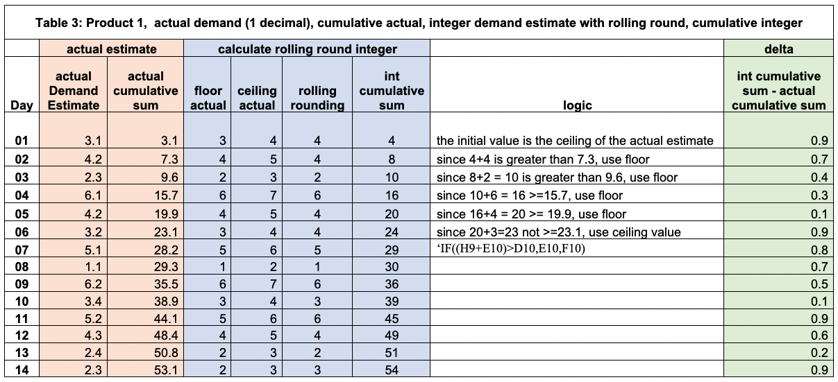
What algorithm do we use to generate integer estimates where the cumulative sum of the integer estimate is always greater than or equal to the cumulative sum of the actuals, and size of delta is never greater than 1? Table 3 demonstrates this algorithm.

1. Day 1, the rolling round estimate is the ceiling (round up), here 3.1  The cumulative sum of the integer estimates for day 1 is 4.
2. Day 2, we add the floor value of the actual estimate (4.2  4) to the cumulative estimate as of day 1 (4) which gives us 8 (=4+4). If this value is greater than or equal to the actual cumulative sum for day 1 (which is 7.3), then we select the floor value and the rolling rounding estimate for day 2. If not, then the ceiling estimate is used.
3. Day 3, 2(floor) + 8 (integer cumulative sum) = 10, which is >= 9.6 (cumulative sum actual), select floor (2).
4. Day 6, 3(floor) + 20 (integer cumulative sum) = 23, which is < 23.1 (cumulative sum actual), select ceiling (4) to use as rolling round estimate for day 6.

Observe in the last column of Table 3, all the values are positive and all less than or equal to 1. 

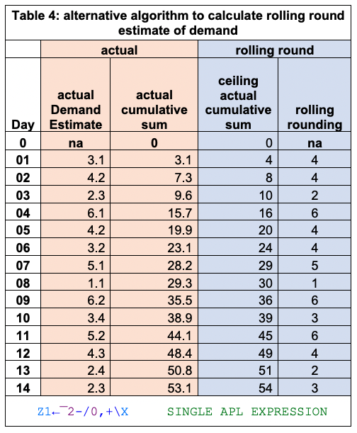
An alternative algorithm is demonstrated in Table 4. Step 1 is calculating the ceiling value for the actual cumulative sum (show in column 4). The rolling rounding estimate (column 5) is the difference between ceiling of actual cumulative sum (column 4) for today with yesterday. The rolling round estimate for day 4 (6) is ceiling for cumulative sum day 4 (16) minus the ceiling of the cumulative sum for day 3 (10); 6 = 16-10. In APL2 the code is “Z1←¯2- /0,⌈+\X”.

Conclusion

In many areas of supply chain management, analytic methods generate estimates with “pesky decimals”. For example, demand estimates and production planning. The traditional method to eliminate pesky decimals is rounding. However, this also results in the loss of critical information; the cumulative sum can often either understate or overstate workload on the firm.  The rolling rounding method caps this information loss at 1.

Enjoyed this post? Subscribe or follow Arkieva on Linkedin, Twitter, and Facebook for blog updates.