I spent some time discussing MAPE and WMAPE in prior posts. In this post, I will discuss Forecast BIAS. Forecast BIAS can be loosely described as a tendency to either
Forecast BIAS is described as a tendency to either
- over-forecast (meaning, more often than not, the forecast is more than the actual), or
- under-forecast (meaning, more often than not, the forecast is less than the actual).
Now there are many reasons why such bias exists, including systemic ones. In this blog, I will not focus on those reasons. Instead, I will talk about how to measure these biases so that one can identify if they exist in their data.
A quick word on improving the forecast accuracy in the presence of bias. Once bias has been identified, correcting the forecast error is generally quite simple. It can be achieved by adjusting the forecast in question by the appropriate amount in the appropriate direction, i.e., increase it in the case of under-forecast bias, and decrease it in the case of over-forecast bias.
Rick Glover on LinkedIn described his calculation of BIAS this way: Calculate the BIAS at the lowest level (for example, by product, by location) as follows:
- BIAS = Historical Forecast Units (Two months frozen) minus Actual Demand Units.
- If the forecast is greater than actual demand than the bias is positive (indicates over-forecast). The inverse, of course, results in a negative bias (indicates under-forecast).
- On an aggregate level, per group or category, the +/- are netted out revealing the overall bias.
The other common metric used to measure forecast accuracy is the tracking signal. On LinkedIn, I asked John Ballantyne how he calculates this metric. Here was his response (I have paraphrased it some):
- The “Tracking Signal” quantifies “Bias” in a forecast. No product can be planned from a badly biased forecast. Tracking Signal is the gateway test for evaluating forecast accuracy. The tracking signal in each period is calculated as follows:
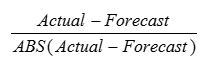
- Once this is calculated, for each period, the numbers are added to calculate the overall tracking signal. A forecast history totally void of bias will return a value of zero, with 12 observations, the worst possible result would return either +12 (under-forecast) or -12 (over-forecast). Generally speaking, such a forecast history returning a value greater than 4.5 or less than negative 4.5 would be considered out of control.
At Arkieva, we use the Normalized Forecast Metric to measure the bias. The formula is very simple.
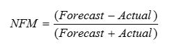
As can be seen, this metric will stay between -1 and 1, with 0 indicating the absence of bias. Consistent negative values indicate a tendency to under-forecast whereas consistent positive values indicate a tendency to over-forecast. Over a 12 period window, if the added values are more than 2, we consider the forecast to be biased towards over-forecast. Likewise, if the added values are less than -2, we consider the forecast to be biased towards under-forecast.
A forecasting process with a bias will eventually get off-rails unless steps are taken to correct the course from time to time. A better course of action is to measure and then correct for the bias routinely. This is irrespective of which formula one decides to use.
Good supply chain planners are very aware of these biases and use techniques such as triangulation to prevent them. Eliminating bias can be a good and simple step in the long journey to an excellent supply chain.
Like this blog? Follow us on LinkedIn or Twitter, and we will send you notifications on all future blogs.