The Relationship Between Forecast Accuracy and Safety Stocks

A company’s total inventory consists of many types of stock such as strategic, anticipation, safety, cycle, and unplanned. Cycle stock is most connected to the demand forecast; it is expected to be sold as the forecast becomes real demand. Safety stock on the other hand is extra stock to deal with the variability of the demand or supply. As such, it is not always linked to forecasting accuracy.

The most common way of calculating the safety stock uses, among other things, the variance of historical demand to calculate the safety stock. Further, it applies a service level factor based on the assumption of the demand being normally distributed. (This assumption has its well-documented limitations which we will not get into here.) The assumption of normal distribution also makes the average demand a good estimate for expected demand in the future.

Learn More: An Approach to Setting Forecast Accuracy Targets

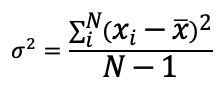
Now, a modern business typically has a better estimate of the expected demand, which is the forecast. Why spend time and money developing a good forecast, only to use the average demand as the estimate of expected demand in the future? One recommendation is that people calculate the variance based on the forecast error and not based on mean demand. This is demonstrated below in terms of the formula of variance, which is the square of standard deviation. If x_i represents the actual demand in period i, then the formula is:

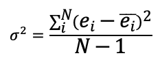
When a company is involved in forecasting, one can calculate the error e_i = x_i – f_i, where x_i, f_i, and e_i represent the actuals, forecast, and the error respectively for period i. The recommended formula for variance then becomes:

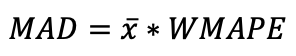
When one uses the second formula, the safety stock is calculated from the forecast error variance. As a result, one can expect that the safety stock values will go up and down as the forecast error goes up and down. There is a theoretical basis to this as well. Standard deviation is related to MAD. Further, MAD is related to WMAPE, which is one way of measuring forecast error. Specifically:

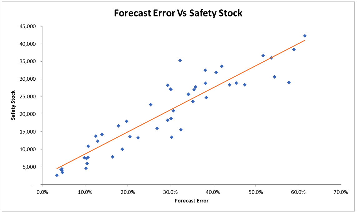
Now, these relationships are dependent on the distribution of the demand data. However, demand streams could have different statistical distributions. Instead of relying on one or another statistical distribution, we decided to test this relationship with data empirically using regression. We calculated the safety stock using the formula above and simulated it with different forecast errors. Below are the results for the first data set.

Learn More: How Forecastable is Your Data?

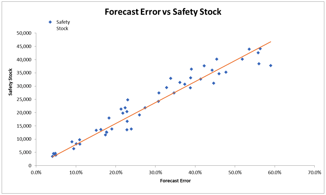
The regression results did show a very strong relationship between safety stock and forecast error with the statistical significance approaching 99.99%.

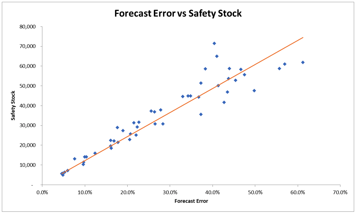
In the above regression, we disallowed the intercept (the constant term). Below are the results when the intercept is included.

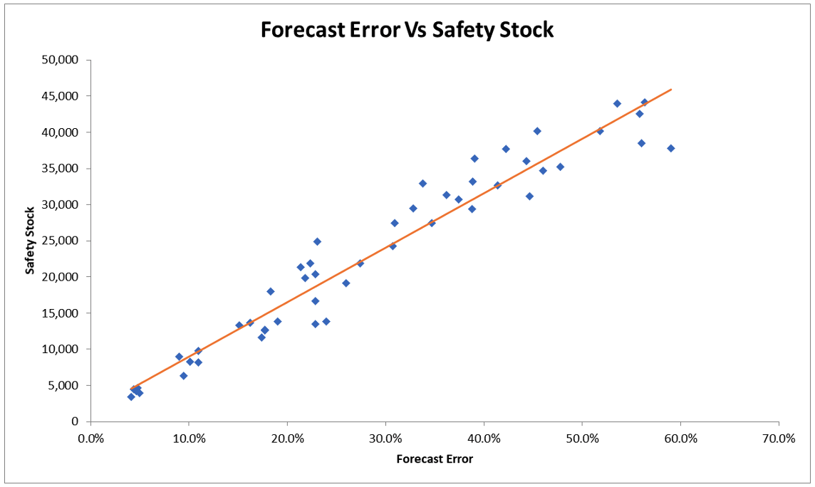
It is worth noting that the intercept was a small amount with a significantly lower statistical significance (by way of the t-statistic). In both cases, the total safety stock has a strong relationship to the forecast error. As forecast error increases, safety stock increases.

Below are the results for two other data sets.

Data set 2: Without Intercept:

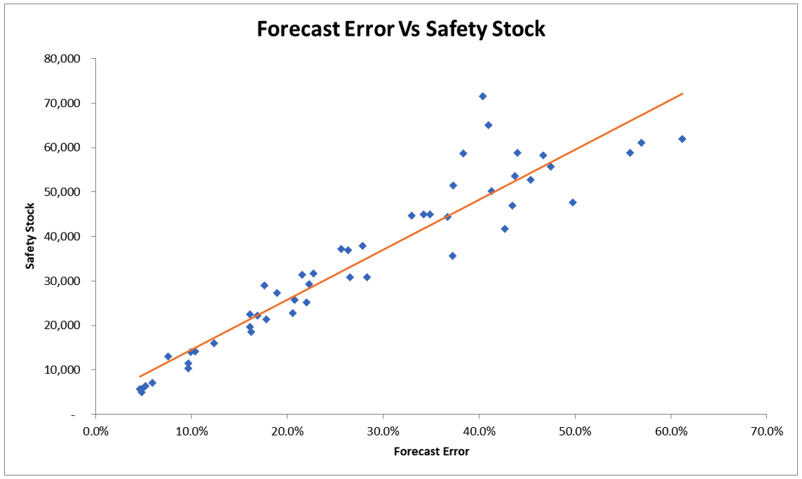
Data set 2: With Intercept:

Data set 3: Without Intercept

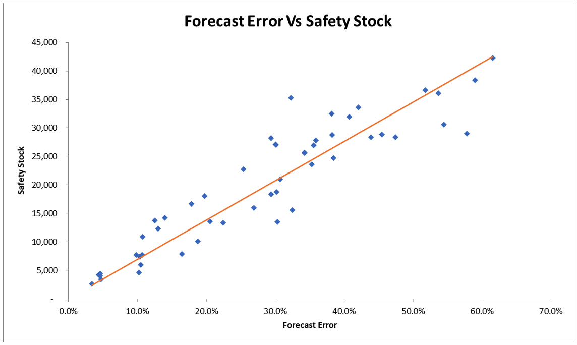
Data set 3: With Intercept

In both data sets 2 and 3, the coefficient of the factor (forecast error) was very significant, just as in data set 1.

This is an interesting, although not completely unexpected, outcome. We strongly encourage practitioners to experiment with calculating safety stock using this formula, especially if they have confidence in their forecast. This will then have an incremental ROI on their demand planning and forecasting.

Do you calculate safety stock using this technique? What has your experience been? Please share in the comments below.